Return the Last Value in a Column with the Offset Function

You can easily Excel find last value in column using the OFFSET function. Just follow the tutorial below and you can fetch that last value. But before you move, let’s first understand how the OFFSET function works!

Key Takeaways

• OFFSET Dynamically References Cells – The OFFSET function allows you to reference a cell based on a starting point and specified row/column offset, making it flexible for dynamic ranges.

• Perfect for Finding Last Value – By combining OFFSET with other functions like COUNTA or COUNT, you can easily reference the last filled cell in a column, regardless of how many entries there are.

• Handles Varying Data Lengths – The OFFSET formula adapts to changing data ranges, making it ideal when rows are frequently added or removed.

• Works Well with Volatile Data – Since OFFSET is a volatile function, it recalculates every time the worksheet changes, ensuring the result is always current.

• Can Be Combined with Other Functions – OFFSET pairs well with functions like INDEX, MATCH, COUNTA, and SUM to create more advanced dynamic formulas.

OFFSET Function Overview

What does it do?

It returns a reference to a range, from a starting point to a specified number of rows, columns, height, and width of cells

Formula breakdown:

=OFFSET(reference, rows, columns, [height], [width])

What it means:

• reference – It is the starting point from which you want to base the offset function. Required
• rows – It is the number of cells you want to go up/down. Required
• columns – It is the number of cells you want to go left/right. Required
• height – It is the number of rows you want the return reference to be. Optional 
• width – It is the number of columns you want the return reference to be. Optional

If you omit the height or width argument, the output will have the same height or width as a reference!

---

The OFFSET function in Excel is one of the Lookup functions and is great if you want to reference a range of cells and use that reference to do a calculation.

Click here to see how the formula works visually & interactively!

Now that you are familiar with offset function, let’s see how excel return last value in column!

 

How to Return the Last Value in a Column with the Offset Function

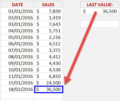
In this example, we have a list that we enter our daily sales into and want to show the last transactional value entered.

This can be used to highlight the latest sales value in a Dashboard or daily metrics report.

=OFFSET

 

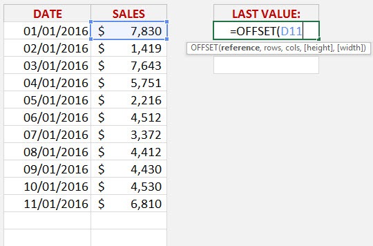
STEP 2: 1st Offset argument – Where do we want to start our reference?

This is at the start of the Daily Sales list:

=OFFSET(D11

 

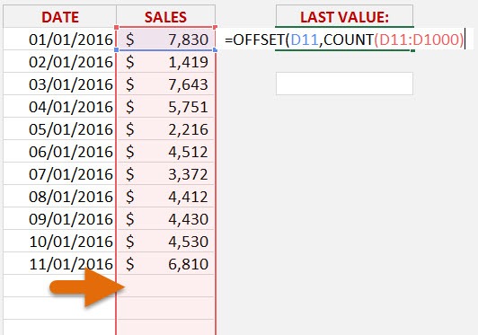
STEP 3: 2nd Offset argument – How many Rows down do we want to go?

This is where the COUNT function is used to count how many transactions we have in our list and go down by that amount.

So as we are starting at cell D11, we are going to go down 11 cells ( COUNTA(D11:D1000) ) and we end up after the last cell with a value.

NB: It is always a good idea to enter an ending range that is more than your last data cell.  That way as your new data get entered, we will be sure to capture it!

=OFFSET(D11, COUNT(D11:D1000)

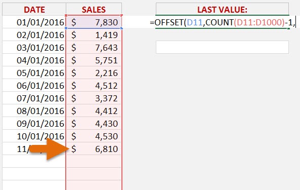
STEP 4: How many of the last sales transactions do we want to Sum?  1

So we need to take away 1 from the COUNT formula which means that our Offset function will go up by 1 cell:

=OFFSET(D11, COUNT(D11:D1000)-1,

STEP 5: 3rd Offset argument – How many Columns to the right/left do we want to move?

We do not want to move to any Columns, so we simply enter 0

=OFFSET(D11, COUNT(D11:D1000)-1,0,

 

STEP 6: 4th Offset argument – How High do we want our referenced data to be?

Since we want to show the last transaction, then we need the [height] to be 1 cell high:

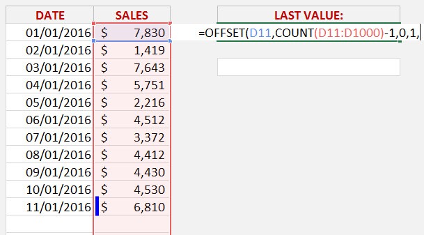
=OFFSET(D11, COUNT(D11:D1000)-1,0,1,

STEP 7: 5th Offset argument – How Wide do we want our referenced data to be?

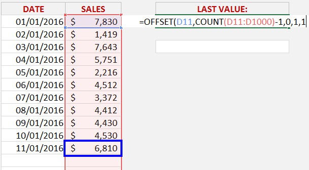
We want to reference 1 Column only, so we need to enter 1 for the [width]

=OFFSET(D11, COUNT(D11:D1000)-1,0,1,1))

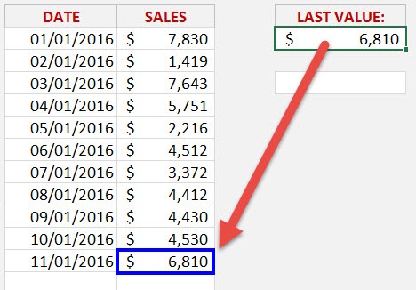
As we can see the Sum of the last transaction from our example is $6,810.

This is how you can use Excel formula last cell in column with data!

This formula is dynamic as well. If we add more transactions at the bottom of our Sales list then it automatically Excel find last value in column, without the need to update the formula 🙂

Let’s try that!

In this example, you have added two additional daily sales data and you will see the value returned by the formula will be updated.

This completes our Excel last value in column using the OFFSET function!

Frequently Asked Questions

How do I use OFFSET to return the last value in a column?
You can use a formula like:
=OFFSET(A1, COUNTA(A:A)-1, 0)
This starts at A1, moves down by the number of filled cells minus one, and returns the last value.

What is the advantage of using OFFSET for finding the last value?
OFFSET allows you to dynamically adjust to varying data lengths without needing to manually update ranges.

Is OFFSET volatile and what does that mean?
Yes, OFFSET is a volatile function, meaning it recalculates whenever any change is made in the worksheet, keeping the result always up to date.

Can I use OFFSET to return the last numeric value only?
OFFSET by itself counts all filled cells (including text), but you can combine it with COUNT instead of COUNTA to count only numeric entries:
=OFFSET(A1, COUNT(A:A)-1, 0)

What are alternatives to OFFSET for returning the last value?
You can also use LOOKUP, INDEX, or XLOOKUP functions to achieve similar results, though OFFSET is preferred for flexible range-based referencing.