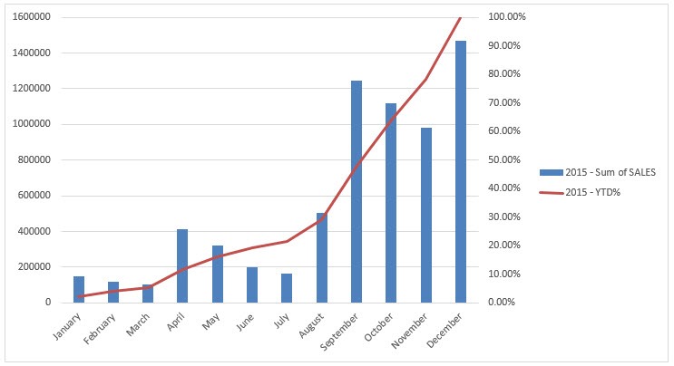
A Running Total In is the accumulation of values over a certain period, like days, month or years. It is sometimes referred to as the Year to Date analysis.
A Running Total In takes one period’s values, then adds a second period, then a third period…and so on, to give the accumulated values up to a certain period.
This can be show in dollar form or in percentage form.
With an Excel Pivot Table we can easily include this calculation without the need to use any formulas. Here is how:
STEP 1: Insert a Pivot Table by clicking in your data and going to Insert > Pivot Table and choose to insert it in a New or Existing Worksheet
STEP 2: You will need to put the Months Field in the ROW area, the Year Field in the COLUMN area and then put the Sales Field in the VALUES area two times!
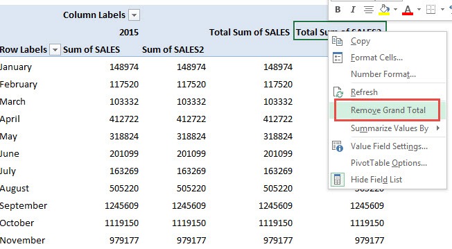
STEP 3: Right Click on a Totals cell and choose Remove Grand Total
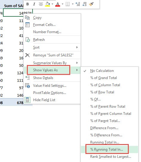
STEP 4: Right Click on a Sum of SALES2 value and select Show Values As > % Running Total In > Base Field: Month
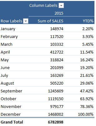
STEP 5: You can manually change the name of the Sum of SALES2 Field by clicking in the cell’s title within the Pivot Table:
STEP 6: We can insert a Pivot Chart by clicking in our Pivot Table and going to PivotTable Tools > Analyze/Options > Pivot Chart
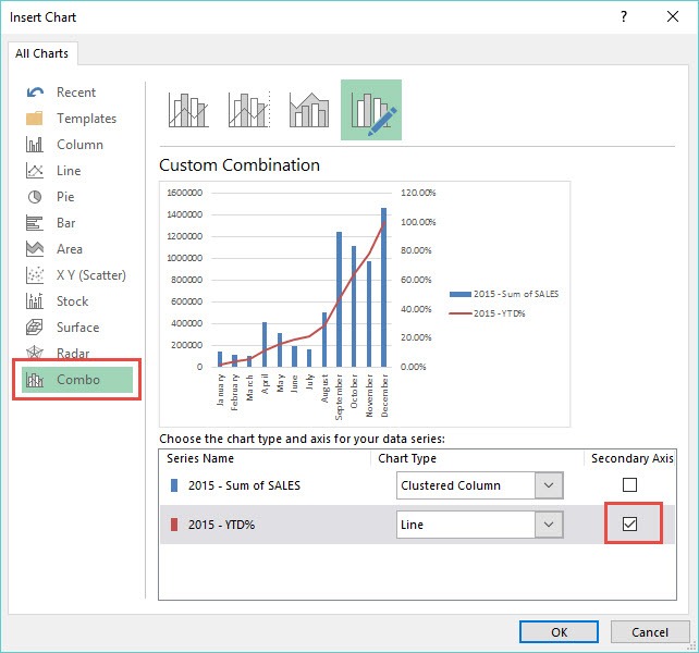
STEP 7: From the Insert Chart dialogue box you need to choose the Combo chart and “check”the Secondary Axis box for the YTD% Series and press OK
You now have your % Running Total In values on a Pivot Table and also shown graphically on a Pivot Chart:
John Michaloudis is a former accountant and finance analyst at General Electric, a Microsoft MVP since 2020, an Amazon #1 bestselling author of 4 Microsoft Excel books and teacher of Microsoft Excel & Office over at his flagship MyExcelOnline Academy Online Course.


