How to Search for a Word in Excel Fast

Searching for a specific word in Excel can save you loads of time, especially when working with large datasets or lengthy spreadsheets. In this article, I’ll walk you through the easiest ways to search for a word in Excel, ensuring you never waste time scrolling endlessly again.

Key Takeaways:

• Excel’s SEARCH function is case-insensitive and allows wildcards, making it flexible for various scenarios.
• Combining SEARCH with other functions like MID, IFERROR, and LEFT enhances data extraction and analysis.
• SEARCH and FIND have distinct capabilities—SEARCH ignores case, while FIND is case-sensitive.
• For handling errors when a word isn’t found, IFERROR ensures clean and interpretable results.
• Advanced search strategies, like using TRIM or splitting data into logical columns, improve accuracy in large datasets.

 

Introduction to Excel’s Search Capabilities

Why Mastering the SEARCH Function Matters

When it comes to Excel, mastering the SEARCH function is akin to unlocking a new level of spreadsheet efficiency. Imagine being able to sift through an entire library of text data with just a few keystrokes. That’s the power of the SEARCH function.

It enables us to quickly locate specific text within a larger string, making it an invaluable tool for data analysis and management. Whether it’s sorting customer feedback, extracting insights from research data, or simply organizing our work, the ability to effectively search text drastically cuts down on the time and effort required.

The Versatility of Text Searches in Excel

Text searches in Excel are incredibly versatile and can be tailored to fit a variety of complex scenarios that go beyond simple data finding. For instance, you can search through voluminous spreadsheets for certain keywords to highlight trends, or you can filter and sort data based on search results to better inform your decisions.

Moreover, Excel’s search functions can be combined with other features—like conditional formatting or pivot tables—to visualize your findings or to further manipulate and analyze your data. The adaptability of text searches transforms Excel from a mere data entry tool to a dynamic program capable of handling sophisticated data-driven tasks.

 

How to Search for a Word in Excel

Understanding the Basic Syntax and Arguments of SEARCH function

Understanding the syntax and arguments of Excel’s SEARCH function is like learning the simple rules of a versatile and powerful tool. The basic syntax for the SEARCH function is quite straightforward:

=SEARCH(find_text, within_text, [start_num])

where find_text is the text you are looking for, within_text is the cell range or text string you’re searching within, and the [start_num] is an optional argument that specifies where in the text to begin the search.

Carefully noting these arguments is crucial as the function’s effectiveness depends on its precise application. For example, an incorrectly referenced cell or missing quotation marks could lead to unwanted errors or results.

The Difference Between SEARCH and FIND

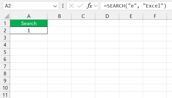
The difference between Excel’s SEARCH and FIND functions is subtle but significant. While both return the location of a specified text within a string, SEARCH is case-insensitive and will disregard whether letters are upper or lower case in its search. For example, SEARCH("e", "Excel") would return 1, finding the first letter ‘E’ even though it’s uppercase.

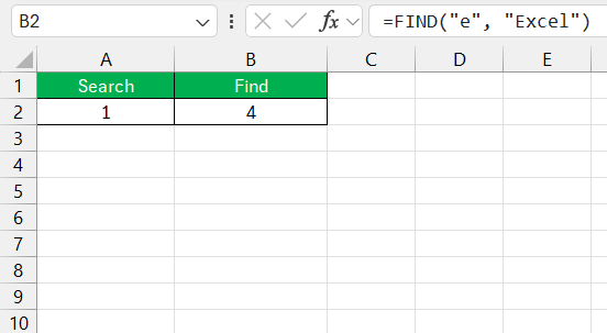
On the other hand, FIND is case-sensitive and pays attention to the text’s case. Using FIND("e", "Excel") would return 4, as it locates the first lowercase ‘e’ in the word.

Additionally, only SEARCH accepts wildcard characters like the question mark (?) to represent a single character and the asterisk (*) for a series of characters, adding a layer of flexibility to your searches.

This distinction is pivotal when working with data where case sensitivity is crucial or when patterns within the text are more important than exact matches.

 

Practical Applications of the SEARCH Function

Extracting Substrings from Cell Data

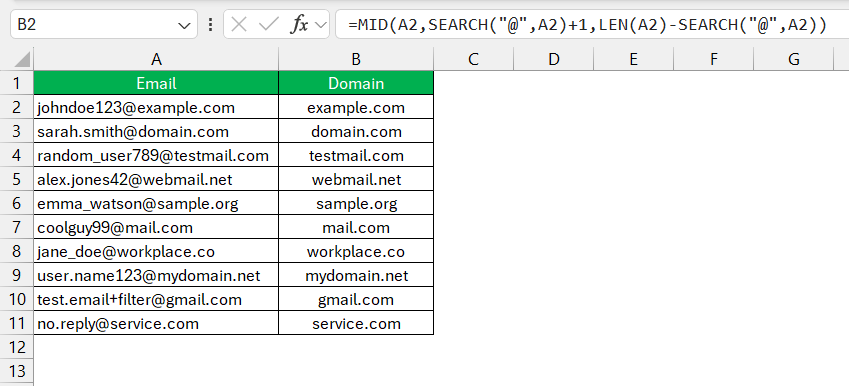
When I need to extract specific portions of data from a cell in Excel, the SEARCH function becomes a key player in my toolkit. Say I’m faced with a long list of product codes or email addresses and I need just a small part of each—a domain name, specific product identifier, or any substring—it’s the SEARCH function combined with MID or LEFT/RIGHT that allows me to isolate precisely the part I need.

For instance, if I want to extract everything after the “@” symbol from an email address, I can use the SEARCH function to find the position of the “@” and then use that as a starting point with the MID function.

This combination transforms a daunting manual task into a streamlined and error-free process.

Determining the Nth Occurrence of a Character

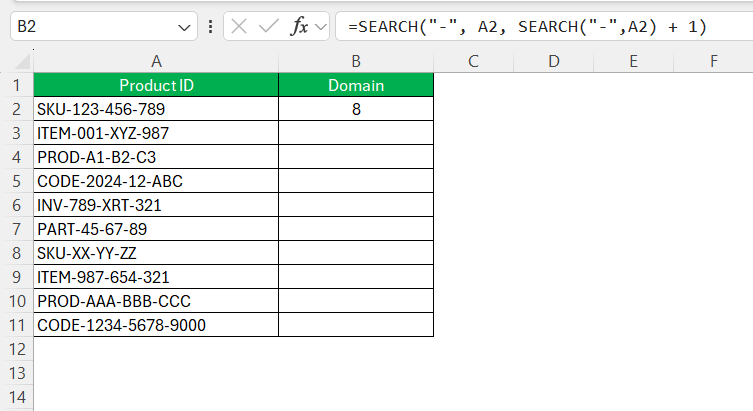
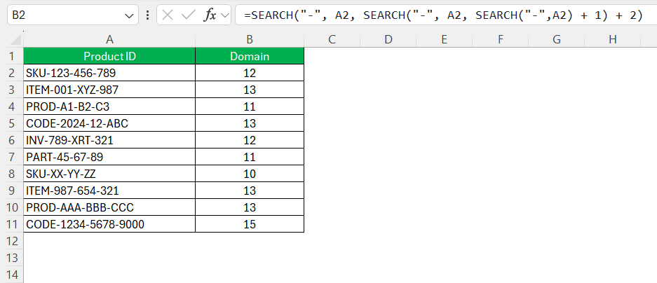
Determining the Nth occurrence of a character in a cell can seem complex, but it’s quite manageable with the right formula. Say I need to find the position of the second dash “-” in an SKU number, I would use a formula that combines the SEARCH function within itself, like so:

=SEARCH("-", A2, SEARCH("-",A2) + 1)

This formula cleverly nests two SEARCH functions where the first one locates the initial dash and the second one begins its search one character after that position. For the third occurrence, it’s a matter of adding another SEARCH layer:

=SEARCH("-", A2, SEARCH("-", A2, SEARCH("-",A2) + 1) + 2)

By incrementing the start number appropriately, I can pinpoint any Nth occurrence within the text string.

Combining SEARCH with Other Functions for Complex Tasks

For more complex tasks, I’ve often found that combining the SEARCH function with other Excel functions can significantly expand my data analysis capabilities. For example, using SEARCH with IF statements helps me create condition-specific results, like flagging cells containing certain keywords.

Additionally, incorporating it within a larger formula involving MID, LEFT, or RIGHT can be advantageous when dealing with data extraction or manipulation.

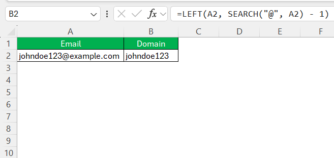
Imagine I want to extract the first word of a cell when it’s followed by a certain character, say a semicolon. Here, I might combine SEARCH to locate the semicolon with the LEFT function to capture everything up to that point:

=LEFT(A2, SEARCH("@", A2) - 1)

Moreover, integrating SEARCH within an IFERROR function ensures that my formulas remain error-free even when the sought-after text is missing, thus keeping the data clean and comprehensive.

 

Troubleshooting Common Issues with SEARCH

Handling Errors When Text Is Not Found

Handling errors gracefully is crucial when the text I’m looking for isn’t found, and this is where good practices come into play. The #VALUE! error crops up when the SEARCH function fails to locate the text, which can happen for a few reasons, such as the search text not being present or starting the search at an index less than one or beyond the length of the text.

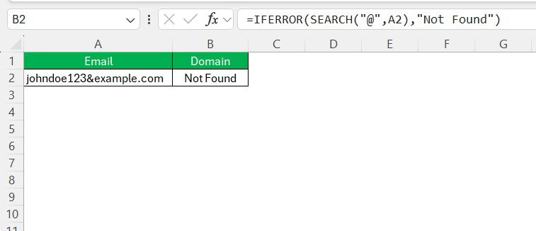
To mitigate this, I utilize the IFERROR function alongside SEARCH. This utility allows me to specify an alternative result when an error would otherwise occur. For instance:

=IFERROR(SEARCH("@", A2), "Not found")

With this, if “@” isn’t found in cell A2, instead of an error, I’ll get a clear “Not found” message. This approach ensures that my datasets remain interpretable and that subsequent analysis is not skewed by cryptic error values.

Tips for Accurate Searching in Large Datasets

When searching large datasets, accuracy is paramount to avoid overlooking crucial information. One tip is to ensure no leading or trailing spaces are skewing my searches, which TRIM can help correct. I also recommend using LOWER or UPPER to standardize case before searching, particularly when combining a case-insensitive function like SEARCH with datasets that might have inconsistent capitalization.

It’s also beneficial to separate data into logical columns whenever possible before searching, as this gives me more control over where I’m searching and reduces the likelihood of mismatches. Last but not least, utilizing Excel’s advanced filtering capabilities in tandem with SEARCH allows for real-time assessment of large volumes of data.

By taking these steps, I can fine-tune my search strategy to effectively manage and analyze even the most extensive datasets.

 

FAQs

What Are the Key Differences Between SEARCH and FIND Functions?

The key differences between SEARCH and FIND functions in Excel are that SEARCH is case-insensitive and allows the use of wildcards, whereas FIND is case-sensitive and does not. This means SEARCH will find a text regardless of its case, and FIND will only locate the text with exact case matching.

How Can I Use the SEARCH Function to Extract Text Between Parentheses?

To extract text between parentheses using the SEARCH function, combine it with MID like this: =MID(A1, SEARCH("(", A1) + 1, SEARCH(")", A1) - SEARCH("(", A1) - 1). This finds the positions of both parentheses and retrieves the substring between them.

Can the SEARCH Function Handle Case-Sensitive Searches?

No, the SEARCH function in Excel cannot handle case-sensitive searches on its own, as it is inherently case-insensitive. For case-sensitive searches, you should use the FIND function instead.

Is It Possible to Search for Multiple Words at Once Using SEARCH?

Yes, it’s possible to search for multiple words using separate SEARCH functions nested within an IF or another logical function, allowing you to test for the presence of several different words or phrases within a cell.

How to do an exact word search in Excel?

To perform an exact word search in Excel and avoid partial matches, you can use wildcard characters with the SEARCH function: prefix and suffix your search term with spaces (e.g., ” myword “) if it’s an interior word or with special characters, parentheses, or separators that may delineate words in your data. If you require a more sophisticated pattern match, consider using regular expressions with VBA for precise control.