I’m used to getting Grand Totals that only show the Total Sum in Pivot Table. But I have a quick hack that allows me to have multiple grand totals! And on top of that, I can customize what value to show. Read on to see how!
Key Takeaways
-
Grand Totals Summarize Key Data Points – Grand Totals in Pivot Tables summarize overall column and row totals, providing a quick view of totals across categories.
-
Enable Grand Totals for Rows and Columns Separately – Excel allows you to turn Grand Totals on or off independently for rows and columns, giving you flexibility in reporting.
-
Multiple Grand Totals for Different Calculations – You can add multiple value fields with different summary functions (e.g., Sum, Average, Count) to display several Grand Totals side by side.
-
Customize Grand Total Labels – You can rename Grand Total labels to make them more meaningful and reflective of the data being summarized.
-
Conditional Formatting Can Highlight Grand Totals – Apply conditional formatting rules specifically to Grand Total rows/columns to make them stand out visually.
Table of Contents
How to Show Multiple Grand Totals
STEP 1: Here is our Pivot Table with multiple Subtotals. However, notice that we only have one Grand Total row.
To know how to insert subtotals in Pivot Table, Click Here.
STEP 2: Go to our data source and add a blank column GRAND TOTAL:
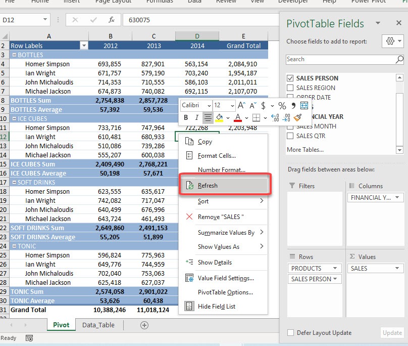
STEP 3: Now right-click anywhere on your Pivot Table and select Refresh
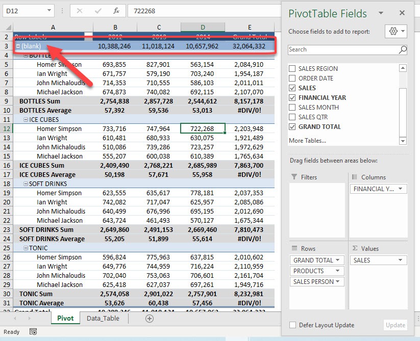
Now the new Grand Total column is now shown there. Drag this to ROWS
You will see our new row being added here.
STEP 4: Press the spacebar and then click on any other cell in the Pivot Table.
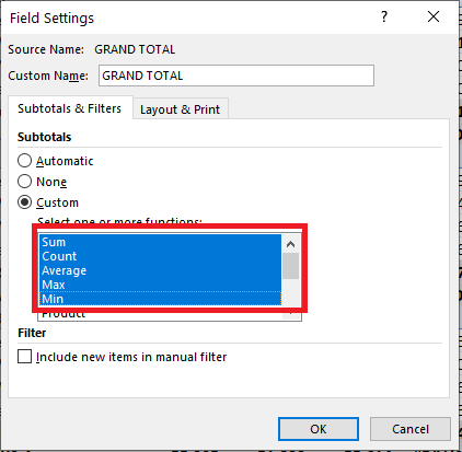
STEP 5: Now let’s do our magic! Right-click on that new row and select Field Settings
Select Custom and pick the functions that you want to display. Click OK.
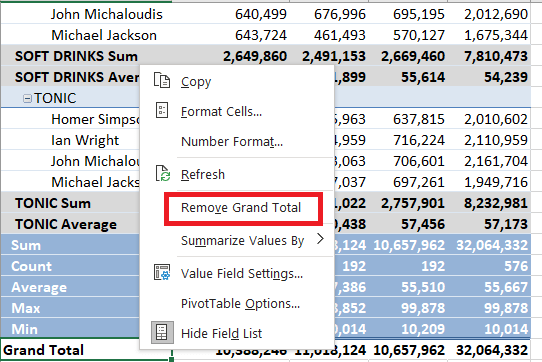
STEP 6: We do not need our Grand Total row anymore. Right-click on it and select Remove Grand Total
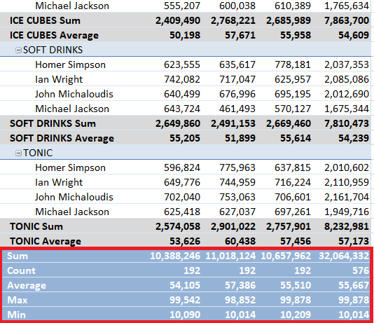
Now you have your multiple Grand Totals!
As you can see, there is no direct way to insert multiple grand totals in Pivot. But you can follow the above mentioned steps and easily insert them in your report.
Frequently Asked Questions
How do I enable Grand Totals in a Pivot Table?
Go to the PivotTable Design tab → Grand Totals → On for Rows and Columns to enable them for both dimensions.
Can I display different types of Grand Totals in the same Pivot Table?
Yes! Simply add multiple value fields and set each one to use a different summary function (like Sum, Average, or Max) to show varied Grand Totals.
How do I rename the Grand Total labels?
Right-click on the Grand Total cell, select “Value Field Settings”, and edit the custom name for clarity.
Is it possible to format only the Grand Total rows/columns?
Yes, apply conditional formatting using rules that target the Grand Total rows or columns specifically.
Can I remove Grand Totals from either rows or columns only?
Absolutely. Under PivotTable Design → Grand Totals, choose either On for Rows Only or On for Columns Only based on your preference.

Bryan
Bryan Hong is an IT Software Developer for more than 10 years and has the following certifications: Microsoft Certified Professional Developer (MCPD): Web Developer, Microsoft Certified Technology Specialist (MCTS): Windows Applications, Microsoft Certified Systems Engineer (MCSE) and Microsoft Certified Systems Administrator (MCSA).
He is also an Amazon #1 bestselling author of 4 Microsoft Excel books and a teacher of Microsoft Excel & Office at the MyExecelOnline Academy Online Course.


