Table of Contents
Introduction to Excel Number Formatting
The Importance of Visual Cues in Data Analysis
Visual cues play an essential role in data analysis by greatly enhancing our ability to quickly understand complex information. When we observe data visually, we process it faster than text or numbers alone. Visual aids like color coding help us detect patterns, trends, and outliers with ease, leading to more efficient decision-making.
In fact, a well-designed spreadsheet that uses color and formatting strategically can be the difference between a good and an exceptional data presentation.
Overview of Excel’s Formatting Capabilities
Excel offers a broad array of formatting capabilities that can transform data into a highly readable and visually engaging format. We’re able to adjust font size, type, and color, apply number formatting like currency or percentages, alter cell background colors, add borders, and much more to make our data stand out.
Excel’s robust toolkit includes conditional formatting, which adapts the formatting based on the data itself, adding a dynamic component to how information is displayed. These formatting options empower us to customize our spreadsheets comprehensively to meet the specific needs of any project.
Quick Guide to Making Negative Numbers Stand Out
Using Conditional Formatting for Instant Recognition
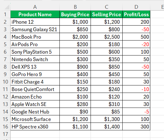
Conditional formatting is a powerful feature in Excel that automatically updates the formatting of cells based on specific conditions. It’s like setting up visual triggers that instantly flag important data. For example, by applying conditional formatting, we can have Excel highlight all negative numbers in red.
This not only makes these figures instantly recognizable but also enables us to track changes in real time, as the formatting will update as soon as the numbers do. By adopting this method, we ensure that our data analysis is both efficient and accurate, as important data points are immediately visible.
Custom Format Approach for Negative Values
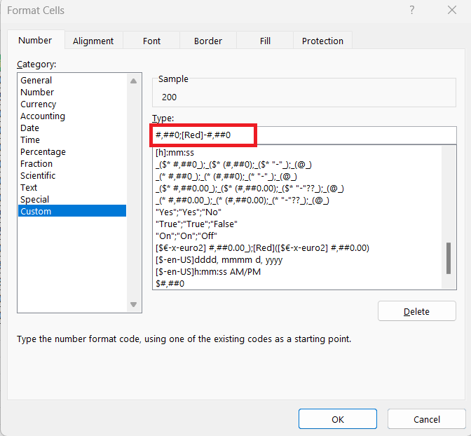
The custom format approach offers a more permanent way to display negative numbers in red throughout an Excel workbook. By creating a custom number format, we tell Excel explicitly how we want positive, negative, zero, and text values to appear. Using a custom format code such as #,##0;[Red]-#,##0, any negative number entered in a cell will automatically turn red, improving readability and consistency within the workbook.
What’s more, this custom format can be saved with the workbook or even as part of a template, making it effortless to preserve our formatting preferences across various documents — a straightforward solution for maintaining visual standards in recurring reports or datasets.
Step-by-Step Instructions for Beginners
Applying Conditional Formatting Rules
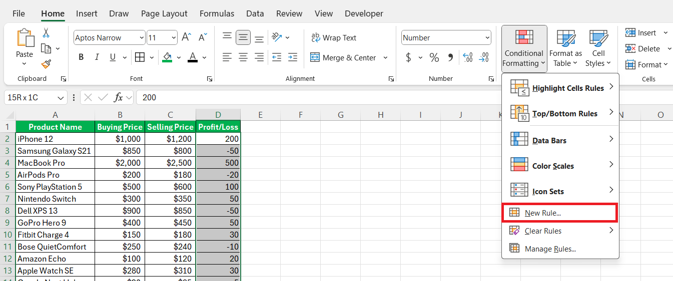
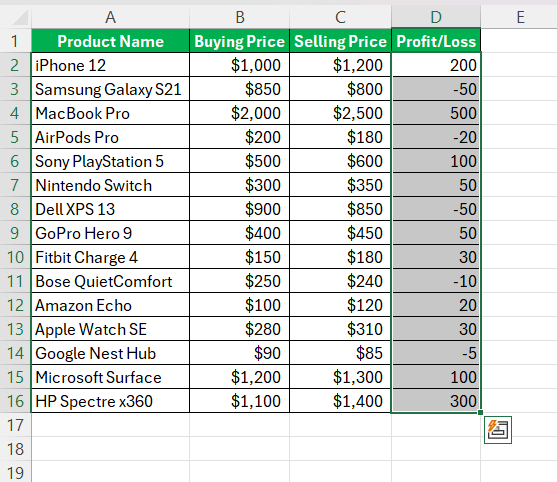
To apply conditional formatting rules, begin by selecting the range of cells you wish to format.
Then, navigate to the ‘Home’ tab and find the ‘Conditional Formatting’ button in the ‘Styles’ group. Choose ‘New Rule’.
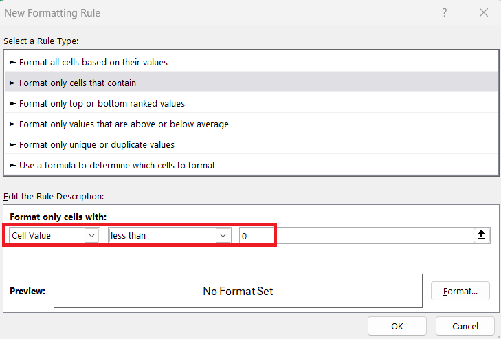
In the dialog box that appears, select ‘Format cells that contain.’ Set the condition for the cell value to ‘less than’ and enter zero.
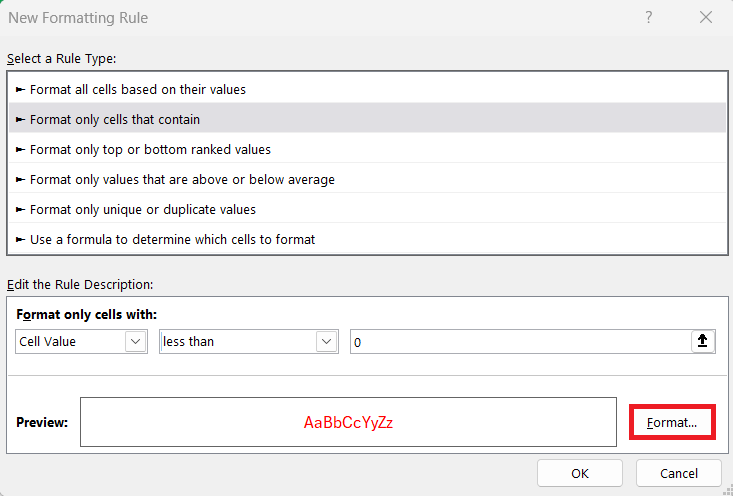
After this, click on ‘Format,’ choose the red color for the font, and confirm by pressing ‘OK.’
With this rule in place, Excel will automatically turn any negative values within the selected range into red text, drawing immediate attention to them.
Creating and Saving Custom Formats
Creating and saving custom formats in Excel is straightforward, even for beginners. To begin, select the cells you want to format.
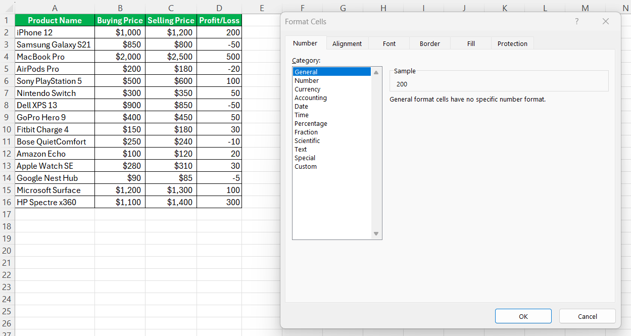
Access the ‘Format Cells’ dialog by right-clicking and choosing ‘Format Cells’ or pressing ‘Ctrl + 1’.
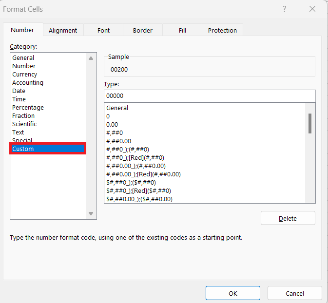
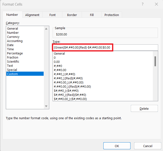
In the dialog, switch to the ‘Number’ tab and select ‘Custom’.
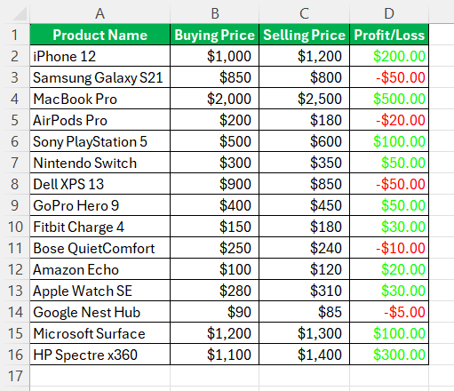
Within the ‘Type’ field, enter a format code that defines the appearance for positive, negative, and zero values, like [Green]$#,##0.00;[Red]-$#,##0.00;$0.00. Once done, click ‘OK’ to apply your custom format.
Your custom format now will not only make negative numbers instantly recognizable but will also save the format within the workbook or a template, ensuring that every time you apply the format, consistency is maintained.
Advanced Tips for Seasoned Excel Users
Crafting Complex Formats with Number and Currency Options
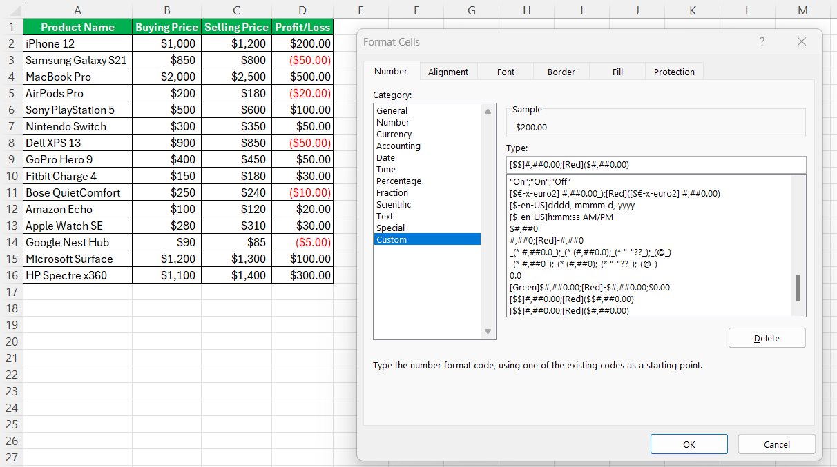
For complex data requirements, crafting formats that handle numbers and currencies can be critical. Advanced Excel users often need to display various formats together, such as differentiating between multiple currency symbols, using accounting formats, or showing negative numbers in parentheses. Excel’s custom format feature allows for such detailed customization.
For instance, to format positive numbers with a dollar sign and negative numbers in red with parentheses, the format code would be [$$]#,##0.00;[Red]($$#,##0.00).
By mastering these complex custom formats, we can make our spreadsheets not only more globally inclusive with currency differentiation but also ensure numbers are displayed precisely to the requirements of financial reporting or other specialized analyses.
Best Practices for Clear Data Presentation
When highlighting negative numbers in Excel, following best practices ensures that your data remains clear and professional. Here are some best practices I adhere to:
1. Consistency Across Worksheets
To maintain uniformity, I apply the same negative number formatting across all worksheets in a workbook. This consistency helps in comparing data and ensures that the visual cue is always the same, regardless of which sheet I’m on.
2. Avoid Overuse of Colors
While red is effective for negative numbers, I avoid overusing colors in my spreadsheets. Too many colors can make the data look cluttered and less professional. I reserve red formatting specifically for negative values to keep the visual focus clear.
3. Combine Formatting with Clear Labels
Negative numbers are more impactful when accompanied by clear labels and headers. I make sure that my columns and rows are well-labeled, so anyone reviewing the spreadsheet can easily understand what the numbers represent, without relying solely on color cues.
4. Document Formatting Choices
For transparency and ease of understanding, I document any special formatting choices in a notes section or a legend within the spreadsheet. This practice helps others (or myself, in the future) understand why certain formatting was applied.
5. Check for Accessibility
I consider accessibility by ensuring that the red color used for negative numbers is distinguishable by people with color vision deficiencies. For critical reports, I might use a combination of color and text formatting (e.g., red text with a minus sign) to improve accessibility.
Tips & Tricks for Effective Formatting
Here are some additional tips and tricks that I find useful for formatting negative numbers and enhancing my Excel spreadsheets:
1. Use Conditional Formatting for Dynamic Changes
If my data changes frequently, I use Conditional Formatting to automatically update the color of negative numbers. This way, I don’t have to manually reapply the formatting each time the data updates. It’s especially useful for large datasets where manual formatting would be cumbersome.
2. Apply Different Formats for Different Contexts
In some cases, I might use different formats for different types of negative values. For instance, I might use a darker red for significant losses and a lighter red for minor losses. This can help in quickly assessing the severity of different issues.
3. Leverage Excel’s Built-In Styles
Excel offers built-in cell styles that include negative number formatting. I often explore these styles as they can provide a quick way to apply professional-looking formats without having to customize everything from scratch.
4. Use Custom Number Formats for Advanced Needs
For advanced formatting needs, I create custom number formats. For example, I might use a custom format to display negative numbers in parentheses (e.g., (1,234.10)) along with a red font. This can be useful in financial statements or reports where such formatting is standard.
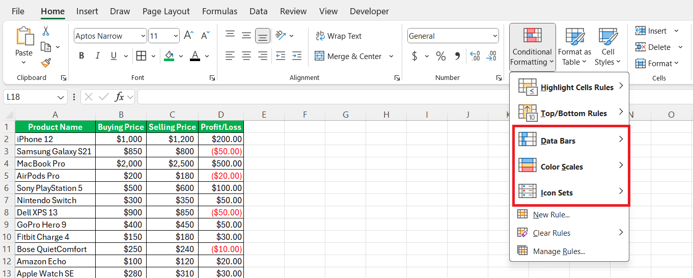
5. Combine with Data Bars or Icons
To add another layer of visual distinction, I sometimes combine red text with data bars or icon sets. Data bars can provide a quick visual reference for the magnitude of negative values, while icon sets can offer additional context at a glance.
6. Save Formatting as a Template
If I frequently use a specific formatting style, I save it as part of an Excel template. This way, I can quickly apply the same formatting to new spreadsheets without having to redo all the settings from scratch.
By following these best practices and incorporating these tips and tricks, I ensure that my Excel spreadsheets are both functional and visually appealing. Proper formatting helps me manage and analyze data more effectively, making it easier to communicate insights and make informed decisions.
Troubleshooting Common Issues When Displaying Negatives
Adjusting Settings When Negative Numbers Do Not Display in Red
If negative numbers are not displaying in red as intended, double-check the applied formatting rules. First, ensure that the conditional formatting rules are set up correctly and applied to the correct cell range. If using custom formats, review the format code in the ‘Type’ box under ‘Custom’ formatting for any errors. Ensure the syntax is correct, for example, use [Red]-General or similar valid codes.
It might also be necessary to check whether the cell is formatted as ‘Text’, as this prevents numerical formats from being applied. If so, convert the text to a number format before re-applying the conditional or custom formatting.
Lastly, if Excel’s options have been modified, it might be affecting how colors are displayed, so resetting Excel’s options to their default can also resolve these issues.
Resolving Custom Formatting Conflicts
Resolving custom formatting conflicts often involves a bit of investigation. Begin by examining if multiple formatting rules are in place that might be overriding each other. Prioritize the order of conditional formatting rules if necessary to ensure the most important rule takes precedence. If using custom number formats, check for any accidental omissions or errors in the format string that could cause a conflict.
Remember, format codes for positive, negative, zero, and text values should be separated by semicolons without spaces. If a conflict persists with other workbook styles or themes, consider removing or modifying those styles to maintain the integrity of your custom formats. Lastly, bear in mind that merging cells or changing cell formatting can also inadvertently affect the custom format, so ensure these actions are not tampering with your intended display.
FAQ Section
How do I apply red formatting to existing negative numbers?
To apply red formatting to existing negative numbers, select the cells, then go to ‘Home’ > ‘Conditional Formatting‘ > ‘Highlight Cells Rules’ > ‘Less Than’. Enter ‘0’ in the box, choose ‘Custom Format’, set the text color to red, and click ‘OK’.
Can I save custom negative number formats for future use?
Yes, custom negative number formats can be saved for future use by creating them in a workbook which you can then save as an Excel template. Next time you need the format, use this template to start your new workbook.
Is it possible to display negative numbers differently based on their value?
Yes, it is possible to display negative numbers differently based on their value by using multiple conditional formatting rules or creating a custom number format with conditions to handle varying ranges of negative numbers.
How do you make negative values red in Excel chart?
To make negative values red in an Excel chart, you must select the data series, right-click, and choose ‘Format Data Series’. Then, under ‘Fill’, use ‘Invert if Negative’ and choose a red color for negative values.
How to format the cell value red if negative and green if positive in excel?
To format cell values red if negative and green if positive in Excel, use conditional formatting. First, select the cells, then go to ‘Conditional Formatting’ on the ‘Home’ tab. Create two rules, one for ‘Less Than’ and one for ‘Greater Than’, and set the formatting to red and green, respectively.
John Michaloudis is a former accountant and finance analyst at General Electric, a Microsoft MVP since 2020, an Amazon #1 bestselling author of 4 Microsoft Excel books and teacher of Microsoft Excel & Office over at his flagship MyExcelOnline Academy Online Course.

