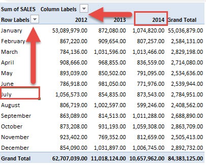
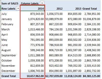
You have your Pivot Table ready, all sorted nicely both from a row and column perspective. However you just need that one minor sorting tweak or two. Well, Excel seemingly has a lot of tricks and you can even sort an Excel Pivot Table manually. For our example, let’s see this Pivot Table below. It is sorted by years (2012-2014), and months (Jan-Dec).
Key Takeaways:
- Drag-and-Drop Sorting: You can manually rearrange rows or columns in a Pivot Table by clicking and dragging the items to the desired order, providing complete control over the display.
- Custom Order for Specific Needs: Manual sorting allows you to organize items in a non-alphabetical or non-numerical order, useful for arranging categories or groups in a way that aligns with specific business needs or priorities.
- Preserving Data Context: Unlike automatic sorting, manual sorting ensures that the context and relationships within the data are maintained, especially when working with grouped or hierarchical data structures.
Table of Contents
How to Sort an Excel Pivot Table Manually
But what if we want to move July to the top, and the year 2014 as the first column year?
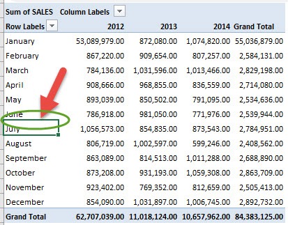
STEP 1: To manually sort a row, click on the cell you want to move. Hover over the border of that cell until you see the four arrows:
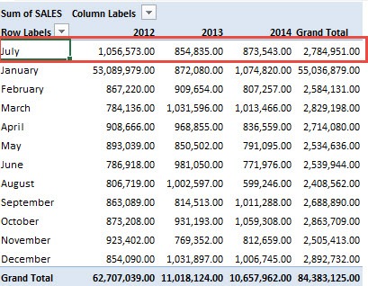
Left mouse click, hold and drag it to the position you want (i.e. upwards to the first row)
We dragged it to the top so it’s now the first row!
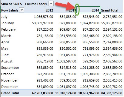
STEP 2: To manually sort a column, click on the cell you want to move. Hover over the border of that cell until you see the four arrows.
Left mouse click, hold and drag it to the position you want (i.e. all the way to the left)
Voila! You have successfully manually sorted your Pivot Table!
EXTRA TIP: You can click inside a cell e.g. January, and start typing in another month, like August. This will also manually sort your Pivot Table items.
Troubleshooting Tips for Pivot Table Sorting Issues
Why Your Pivot Table Sort Might Not Work on Refresh
Have you ever refreshed your pivot table only to find your new data jumbled? It can be disheartening to see your meticulously compiled pivot table disobeying the expected order. This glitch often occurs when adding or updating records. Modern Excel versions are less prone, yet it’s an issue to stay vigilant about. Simply reapplying the sort to pivot table labels should right this wrong. Remember to check if the sorting preference is set to automatic rather than manual; this ensures newly updated items seamlessly find their rightful place.
Resolving Common Pitfalls in Pivot Table Sorting
If you’re entangled in a pivot table sorting snafu, don’t fret! Common issues crop up like unwelcome guests—here are practical fixes you can employ. First, banish any leading spaces in your data to prevent awkward sorting sequences. Check for subtle discrepancies, such as case-sensitive text entries you can’t conventionally sort. Keep in mind that sorting by format or conditional formatting icons isn’t within pivot tables’ native abilities. When you need more muscle for your sort, consider pivot table sorting macros for complex tasks. By being meticulous with your data preparation and understanding Excel’s sorting rules, you can tame unruly pivot tables into submission.
Final Thoughts: Why Master Manual Sorting Matters
Improving Efficiency with Proper Sorting
Proper sorting in pivot tables isn’t just about neatness—it’s the portal to speedier insights and a more intelligent data analysis process. By sorting your data effectively, you not only hasten the journey to conclusions but also make it easier to spot trends, outliers, or critical business indicators. Imagine unearthing sales anomalies with a quick sort by values or aligning customer priorities through a custom order. This isn’t just a skill; it’s an asset that lets you harness the full potential of your data. With each sort, pivot tables transform from sheets of numbers to storytellers, revealing the narratives hidden within your datasets.
Conclusion – The Impact of Sorting Skills on Excel Proficiency
Mastering the art of sorting in Excel’s pivot tables doesn’t just make your data look organized; it cements your status as a proficient Excel user. The ability to swiftly maneuver through complex datasets and extract meaningful patterns is indicative of your Excel mastery. Moreover, your sorting skills can be the difference between an average report and a powerful analytical tool. Remember, in the realm of Excel, proficiency isn’t just about what you do—it’s about how elegantly and efficiently you do it.
Frequently Asked Questions
How do I manually change the order of Columns in a PivotTable?
To manually change the order of columns in a PivotTable, click on the column label you wish to move. Then, press and hold the left mouse button and drag it to your desired position. Release the mouse button to drop the column in its new location. This works great for customizing the view to your preference or emphasizing important data.
How Do I Sort A Pivot Table Left To Right Instead Of Top To Bottom?
Sorting a pivot table horizontally is a snap! Simply right-click on a cell within the row that has the values you’d like to sort. From the context menu, select ‘Sort’, then ‘More Sort Options’. Choose ‘Left to Right’ under the orientation and pick your desired sort order. After selecting the sorting criteria, hit ‘OK’ and voilà – your pivot table now flaunts a horizontal sort!
Can You Set A Custom Order For Sorting Pivot Table Labels?
Absolutely, setting a custom order for pivot table labels is doable and quite handy. Excel’s custom lists allow you to define a specific sequence that defies the standard A to Z or numerical order. For instance, if you have a list with specific priorities or categories that don’t alphabetically sort, a custom list is your ally. Create the list once, and Excel remembers it, making future sorting a breeze as it’ll automatically apply your custom order to relevant pivot table labels.

Bryan
Bryan Hong is an IT Software Developer for more than 10 years and has the following certifications: Microsoft Certified Professional Developer (MCPD): Web Developer, Microsoft Certified Technology Specialist (MCTS): Windows Applications, Microsoft Certified Systems Engineer (MCSE) and Microsoft Certified Systems Administrator (MCSA).
He is also an Amazon #1 bestselling author of 4 Microsoft Excel books and a teacher of Microsoft Excel & Office at the MyExecelOnline Academy Online Course.
