Top 3 Methods to Find Special Characters in Excel

To achieve clean data, finding and managing these special characters can be crucial. These characters might need to be located to ensure consistent and accurate data management.

In this article, we will cover the following topics in detail –

Let us explore these methods one by one!

 

Download the Excel Workbook below to follow along and understand how to find special characters in Excel –

download excel workbookFind-Special-Character-in-Excel.xlsm

 

Method 1 – Using Search Function

We need to use a combination of functions to check the presence of special characters in Excel. In this example, we will be using SUMPRODUCT, ISNUMBER, and SEARCH functions to achieve the desired result.

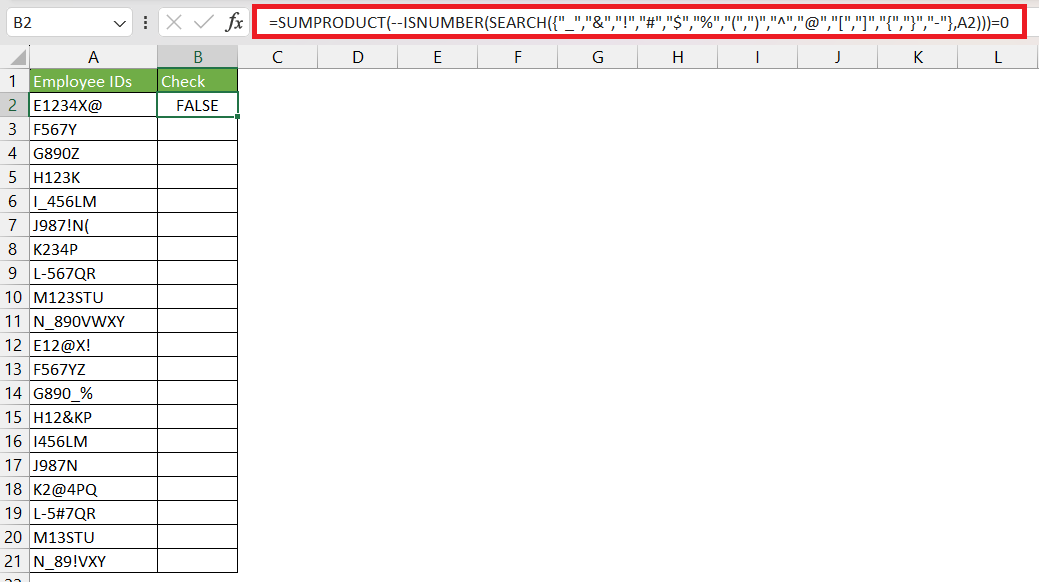
In this example, we have a list of employee IDs that need to be cleaned. Employee IDs should only contain alphabets, numbers. We need to check which of the employee IDs are correct and which are not. Incorrect IDs would contain all special characters like “#”, “-“, “&”, “_”, “!”, “@”, “^”, and “$”.

Follow the steps below to find special characters in Excel –

STEP 1:  Enter the SEARCH function with two arguments –

1. The first argument is all the special characters (within quotes, separated by comma and enclosed in curly brackets)
2. The second argument is the cell containing the text i.e. A2

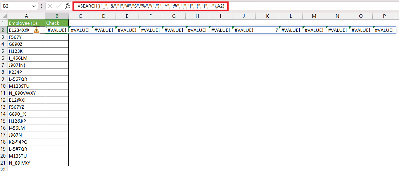
=SEARCH({“_”,”&”,”!”,”#”,”$”,”%”,”(“,”)”,”^”,”@”,”[“,”]”,”{“,”}”,”-“},A2)

This formula will search the content of cell A2 for any of the specified special characters enclosed in the curly braces and return the position of the first occurrence of each character. If no match is found, it returns an error.

STEP 2:  Enter the ISNUMBER function.

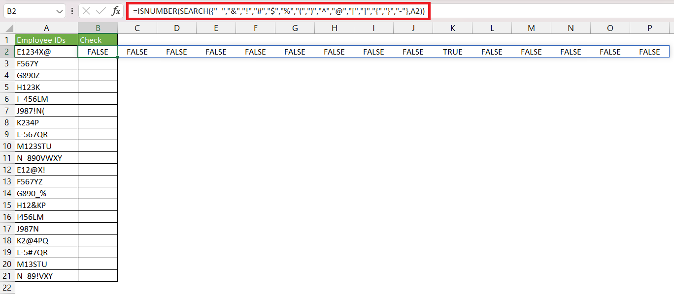
=ISNUMBER(SEARCH({“_”,”&”,”!”,”#”,”$”,”%”,”(“,”)”,”^”,”@”,”[“,”]”,”{“,”}”,”-“},A2))

This function will return TRUE if a match is found (i.e., the position of the special character is a number), and FALSE if no match is found.

STEP 3:  Enter the double minus sign (–) in front of the ISNUMBER function.

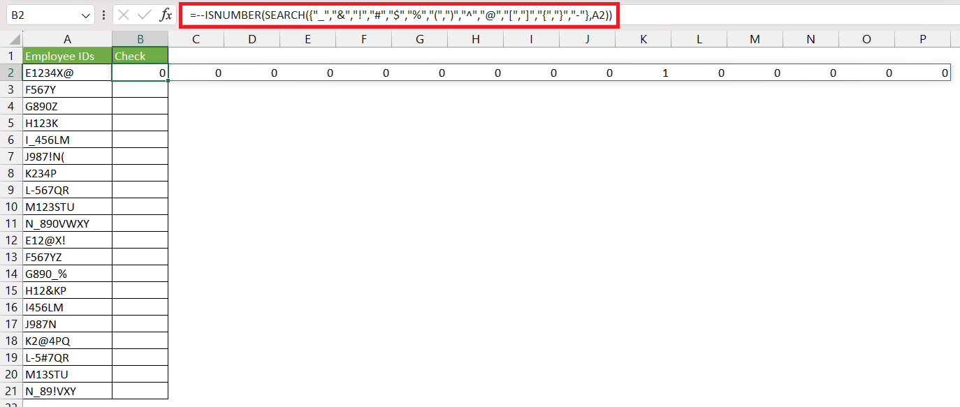
=–ISNUMBER(SEARCH({“_”,”&”,”!”,”#”,”$”,”%”,”(“,”)”,”^”,”@”,”[“,”]”,”{“,”}”,”-“},A2))

This function will convert the Boolean values into 1s and 0s. So, TRUE becomes 1, and FALSE becomes 0.

STEP 4:  Enter the SUMPRODUCT function.

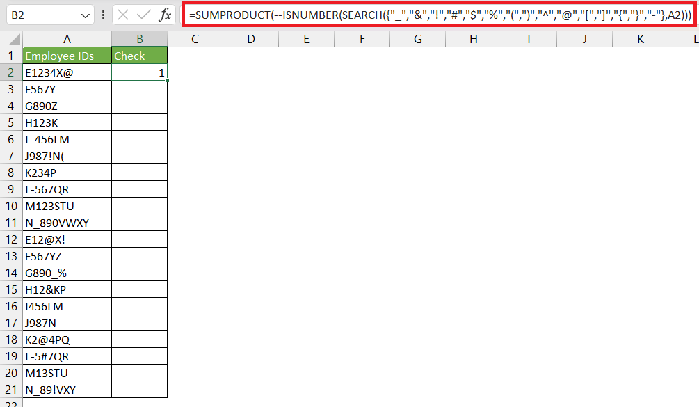
=SUMPRODUCT(–ISNUMBER(SEARCH({“_”,”&”,”!”,”#”,”$”,”%”,”(“,”)”,”^”,”@”,”[“,”]”,”{“,”}”,”-“},A2)))

This function will add up all the 1s and 0s from the previous step.

STEP 5:  Enter “=0” at the end of the formula.

=SUMPRODUCT(–ISNUMBER(SEARCH({“_”,”&”,”!”,”#”,”$”,”%”,”(“,”)”,”^”,”@”,”[“,”]”,”{“,”}”,”-“},A2)))=0

If the summation is equal to zero that means there are no special characters in the contents of cell A2, the function will return TRUE. If there is at least one of the specified special characters found in the cell content, the function will return FALSE.

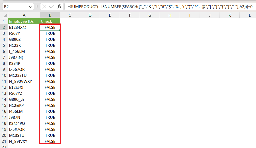
STEP 6:  Copy the formula down.

If the cell contents are free from any of the specified characters then the function will return TRUE or else it will return TRUE.

 

Method 2 – Using User Defined Function

As Excel lacks a dedicated function for locating special characters, we can create one to do the task. We can easily create a User Defined Function to find special characters in Excel by following the steps below –

STEP 1:  Go to Developer Tab > Visual Basic.

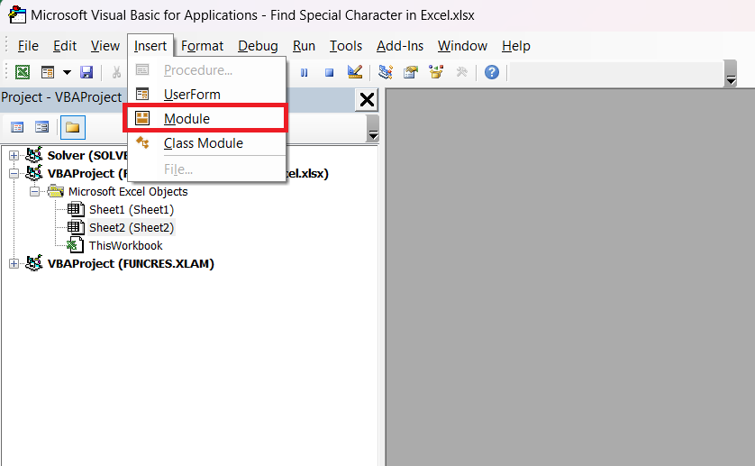
STEP 2:  Go to Insert > Module.

STEP 3:  Enter the code mentioned below –

Public Function Check(inputString As String) As String
Dim length As Long
Dim charAtIndex As String
Check = "Correct"

For length = 1 To Len(inputString)
charAtIndex = Mid(inputString, length, 1)
If charAtIndex Like "[0-9a-zA-Z]" Then
Else
Check = "Incorrect"
Exit Function
End If
Next length
End Function

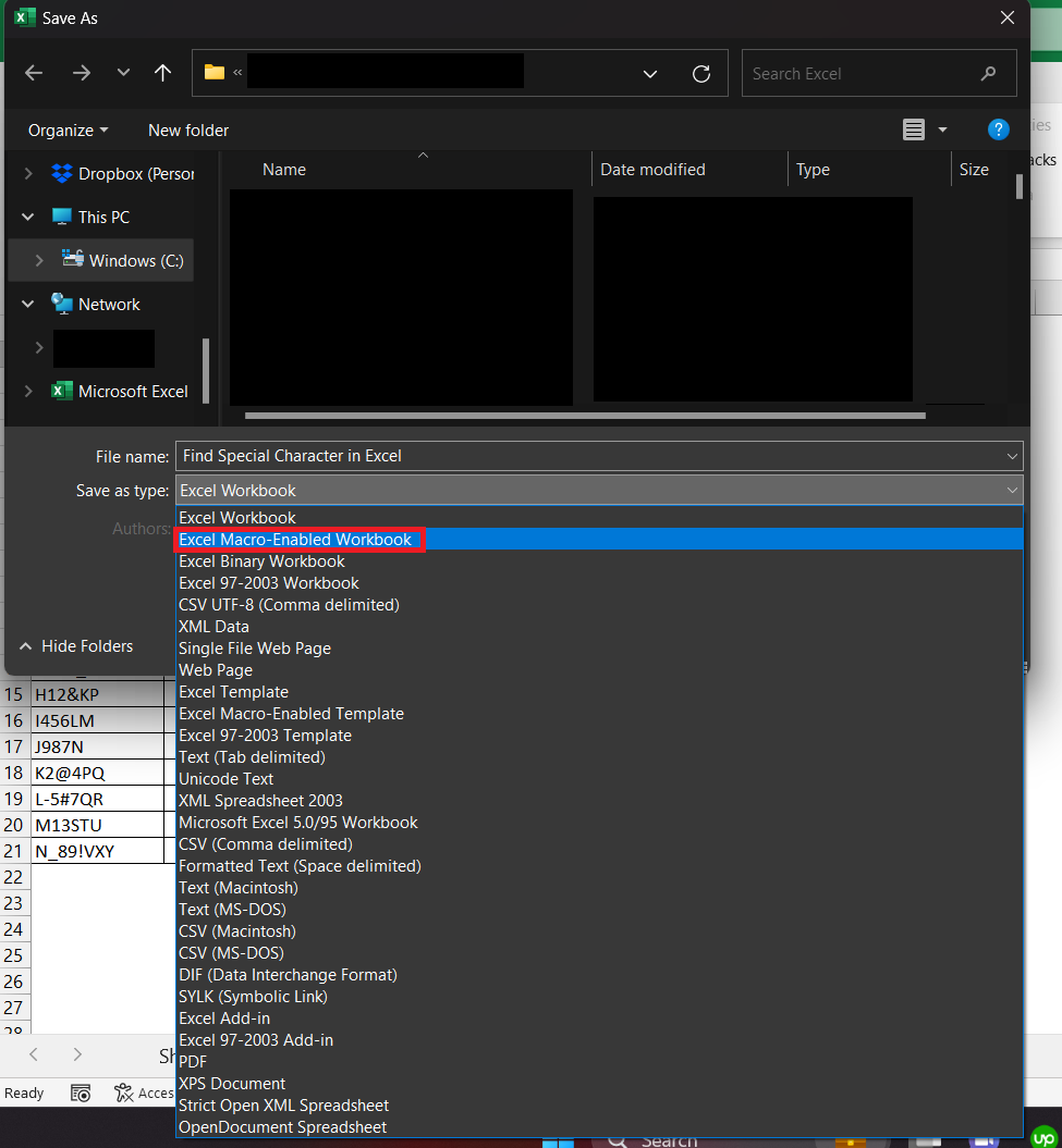
STEP 4:  Press Ctrl + S to save the file as a macro-enabled workbook. Click No.

STEP 5:  In the drop-down, select Excel Macro Enabled Workbook.

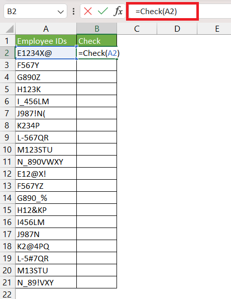
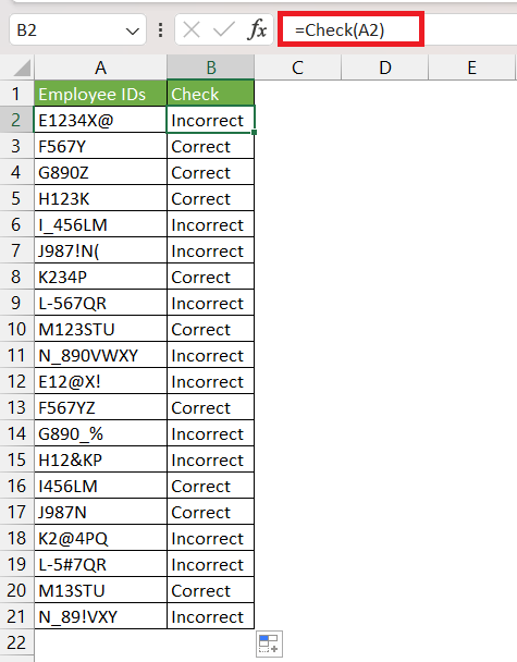
STEP 6: Enter the Check function with cell A2 as the argument.

Here, the function will display “Correct” when the contents of the cell contain only alphabet and letters and “Incorrect” when it contains special characters.

 

Method 3 – Using Power Query

Excel’s Power Query is a robust tool that lets you perform data transformations without complex formulas or manual work. It’s like a game-changer for managing data, and can also be used to find special characters.

Power Query can be used to locate and remove special characters from the contents of the cells. Follow the steps below to achieve the same –

STEP 1: Go to Data > From Table/Range.

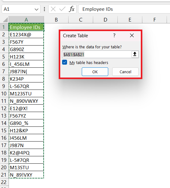
STEP 2: In the Create Table dialog box, select the data and press OK.

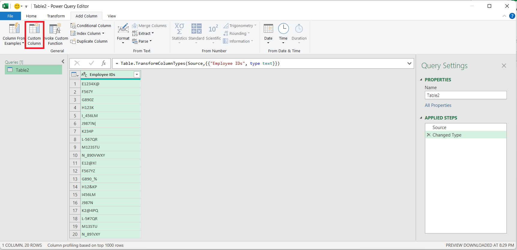
STEP 3: Go to Add Column > Custom Column.

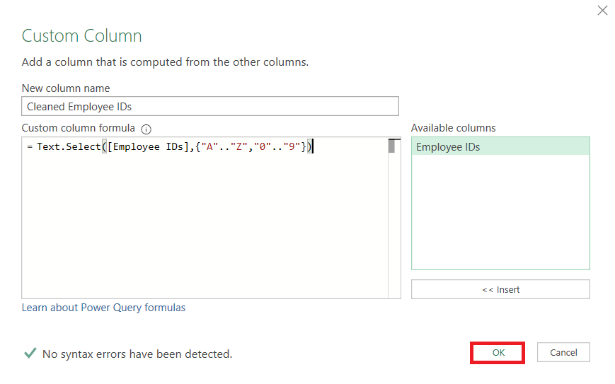
STEP 4: In the Custom Column dialog box, enter –

• Cleaned Employee IDs as New column name.
• =Text.Select([Employee IDs],{“A”..”Z”,”0″..”9″}) as Custom column formula.

Press OK.

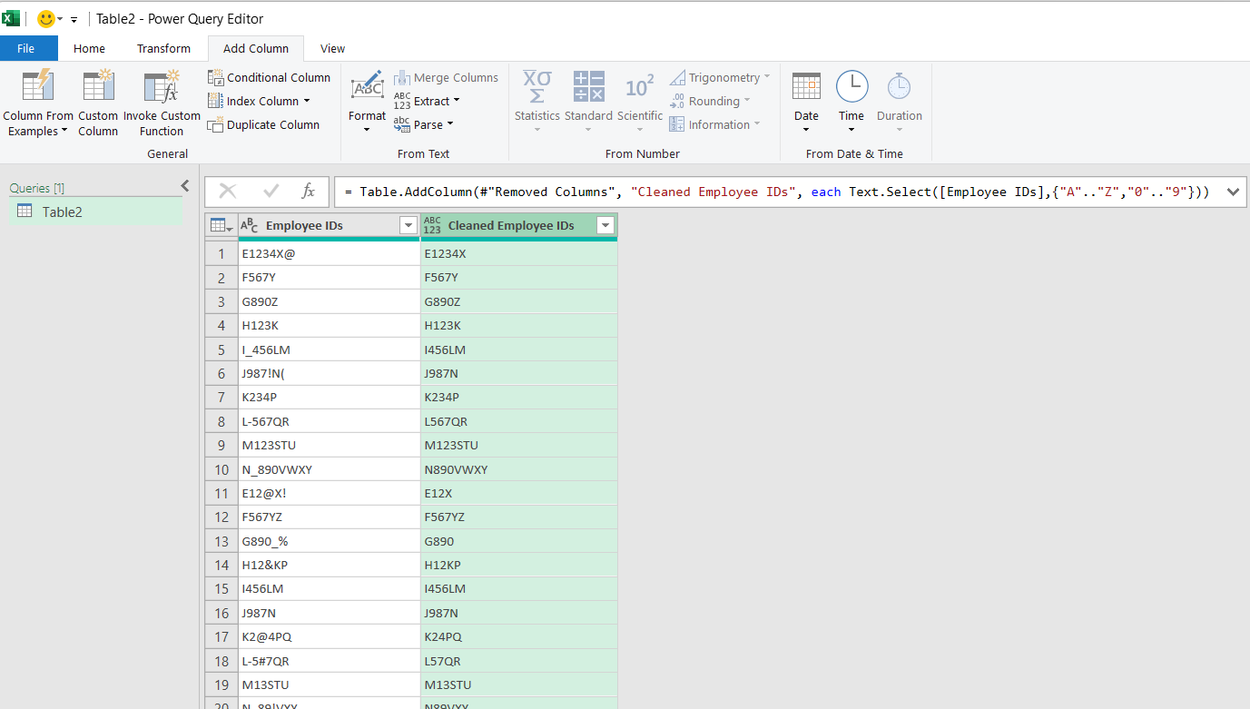
A new column with cleaned data containing only alphabets and numbers will be added.

STEP 5: Go to Home > Close & Load.

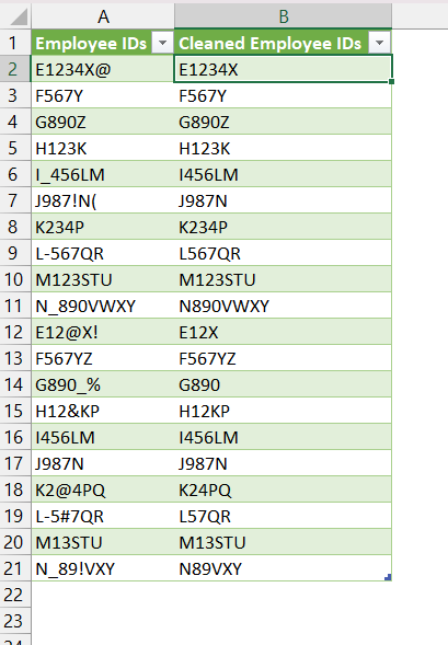
The table will now be added as a new worksheet in the file.

Now, Employee IDs are free from special characters, making them suitable for sorting, filtering, and other data operations without any hindrance.

 

Conclusion

When importing large datasets into Excel, special characters like symbols and signs can appear, making data handling complex. By embracing the techniques mentioned above, data cleanliness and efficient processing can be achieved

To address this, we can use a combination of SUMPRODUCT, ISNUMBER, and SEARCH functions to locate special characters. Another method includes creating a User-Defined Function (UDF) and the third method is to use Power Query.

Further Learning:

• Turn Text To Values With Paste Special Values
• Find Errors with Go to Special Constants
• How to use OFFSET Function in Excel

Click here to learn more about the data cleaning function in Power Query.