Std Dev in Excel Pivot Tables

It is very easy to use a Pivot Table to summarize data for you by giving the sum, count, or average. But did you know it can give you the standard deviation and variance as well? This is crucial if you want to understand how volatile your data is!

Let us explore how to get the std dev in Pivot Table, this shows the amount by which members of a group are different from the average value for the group.

Key Takeaways:

• Standard Deviation Calculation in Pivot Tables – Excel Pivot Tables allow you to calculate standard deviation using StdDev (sample standard deviation) and StdDevP (population standard deviation) as summary functions.
• Choosing the Right Standard Deviation Option – Use StdDev when working with a sample of data and StdDevP when analyzing the entire population to ensure accurate statistical insights.
• Applying Standard Deviation in Value Field Settings – To calculate standard deviation, right-click on the Pivot Table values, select Summarize Values By, and choose either StdDev or StdDevP based on your dataset.
• Interpreting Standard Deviation Results – A higher standard deviation indicates more variability in the data, while a lower value suggests that data points are closer to the average.
• Combining Standard Deviation with Conditional Formatting – You can highlight values that deviate significantly from the mean by applying conditional formatting to standard deviation results, making it easier to analyze trends and outliers.

How to Use Std Dev in Excel Pivot Tables

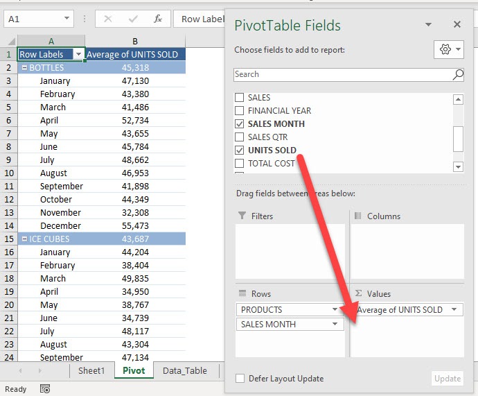
STEP 1: Here is our Pivot Table. Drag UNITS SOLD to the Values Area

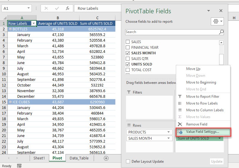
STEP 2: This will default to Sum of UNITS SOLD. Let us change that by clicking on the arrow and selecting Value Field Settings

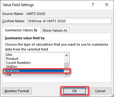
STEP 3: Select StdDevp and click OK.

We will use the StdDevp function as we have the complete data (population) used in the calculation. When only a portion of the data is used, then StdDev should be used instead.

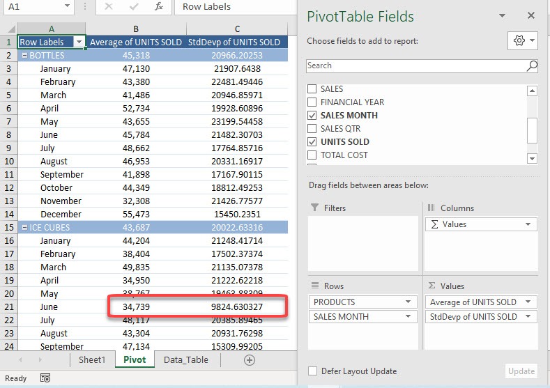
Now you have your Standard Deviation! You can see for ICE CUBES on the month of June the Standard Deviation is quite low. This means that the values on the units sold for that month is fairly close to the average of 34,739.

Frequently Asked Questions

What is the standard deviation function in Excel Pivot Tables?

The standard deviation function in Excel Pivot Tables calculates how spread out the values are from the mean. You can use StdDev for a sample of data or StdDevP for an entire population, depending on your analysis.

How do I calculate standard deviation in a Pivot Table?

To calculate standard deviation in a Pivot Table, add your data to the Values area, right-click on the field, and select Summarize Values By. Then choose either StdDev or StdDevP to apply the desired standard deviation calculation.

What’s the difference between StdDev and StdDevP in Excel?

StdDev is used for sample data, calculating the standard deviation based on a subset of the population, while StdDevP calculates standard deviation for the entire population, using all data points available.

Can I use standard deviation in Excel Pivot Tables with multiple fields?

Yes, you can apply the standard deviation function to multiple fields in a Pivot Table. Simply drag different fields to the Values area and select StdDev or StdDevP for each to analyze their respective standard deviations.

How do I interpret the standard deviation result in my Pivot Table?

A high standard deviation means that your data points are spread out from the mean, indicating high variability. A low standard deviation suggests that the data points are clustered closely around the mean, indicating low variability.

Did you know that the square of the standard deviation will give you the variance value? Click here to know more!

Bryan

Bryan Hong is an IT Software Developer for more than 10 years and has the following certifications: Microsoft Certified Professional Developer (MCPD): Web Developer, Microsoft Certified Technology Specialist (MCTS): Windows Applications, Microsoft Certified Systems Engineer (MCSE) and Microsoft Certified Systems Administrator (MCSA).

He is also an Amazon #1 bestselling author of 4 Microsoft Excel books and a teacher of Microsoft Excel & Office at the MyExecelOnline Academy Online Course.