Strikethrough Shortcut for Mac & Windows in Excel – Step by Step Guide
Introduction to Strikethrough in Excel.
Understanding the Role of Strikethrough in Data Management.
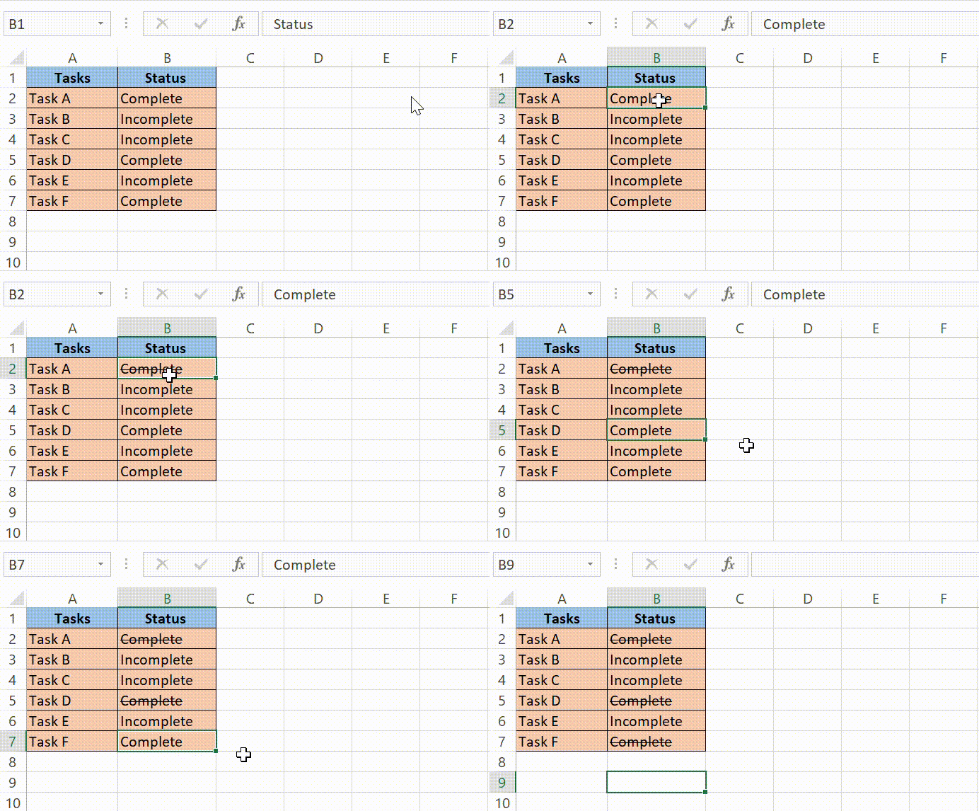
In the world of spreadsheets, strikethrough isn't just for show—it's a secret messenger.When you spot text with a line scored cleanly through it in Excel, it signals that you're looking at tasks wrapped up with a bow or items that have sashayed off the must-have list.
With a glance, this detail distinguishes the done from the do, or the outdated from the updated.
It's a nifty tracker for changes without altering the historical script of your data-driven narrative.
Think of strikethrough as your data's way of saying, "Been there, done that," without losing its place in the story.
Introduction to Strikethrough in Excel
Understanding the Role of Strikethrough in Data Management
In the world of spreadsheets, strikethrough isn’t just for show—it’s a secret messenger. When you spot text with a line scored cleanly through it in Excel, it signals that you’re looking at tasks wrapped up with a bow or items that have sashayed off the must-have list. With a glance, this detail distinguishes the done from the do, or the outdated from the updated. It’s a nifty tracker for changes without altering the historical script of your data-driven narrative. Think of strikethrough as your data’s way of saying, “Been there, done that,” without losing its place in the story.
Differences Between Mac and Windows Excel Versions
When you’re juggling between Mac and Windows, you’ll notice each has its own spin on Excel, making the transition between them a bit like learning dialects of the same language. For starters, Windows loves its control key, while Mac is partial to the command key. This means shortcuts will often use similar key combinations but with a platform-specific twist.
In Windows, you’re living in a world where “Ctrl” is the master key to shortcuts, and strikethrough is no exception. Meanwhile, Mac users rely heavily on the “Command” key in their Excel adventures. The interface and menus can vary slightly, too, with options and features positioned in bespoke locations dictated by the operating system’s design language.
This subtle interplay between the two versions means that, while the core functions remain reliably consistent, the way you interact with them might take some getting used to as you switch from one to the other.
Mastering Strikethrough Shortcuts for Windows Users
Keyboard Shortcut to Apply Strikethrough in Excel for Windows
If you’re working with Excel on a Windows machine, the strikethrough shortcut is like the superhero of keyboard commands—it’s quick, effective, and saves the day in a pinch. Whenever you need to cross out some text, simply select the cell or the specific text within the cell, and summon the strikethrough with a swift Ctrl + 5.
The text in question will wear a neat line across its middle in a blink, marking the task complete or the item obsolete. This keyboard incantation is as simple as it gets, saving you the journey through the labyrinth of menus and settings.
Whether you’re dealing with a solitary cell or a swath of them, this keystroke is your trusty sidekick, ready to dash across your data with the speed of light (or at least as fast as you can press two keys).
Adding a Strikethrough Button to the Quick Access Toolbar
If you find yourself reaching time and again for that strikethrough format, it’s a smart move to give it a permanent home. You can add a strikethrough shortcut button right to the Quick Access Toolbar (QAT) in Excel for Windows, ensuring it’s just a click away.
Let’s carve that pathway to quick strikethrough access:
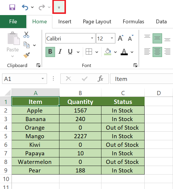
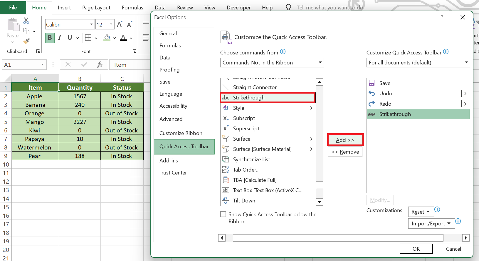
STEP 1: Click the small downward-pointing arrow located at the very top of the Excel window.
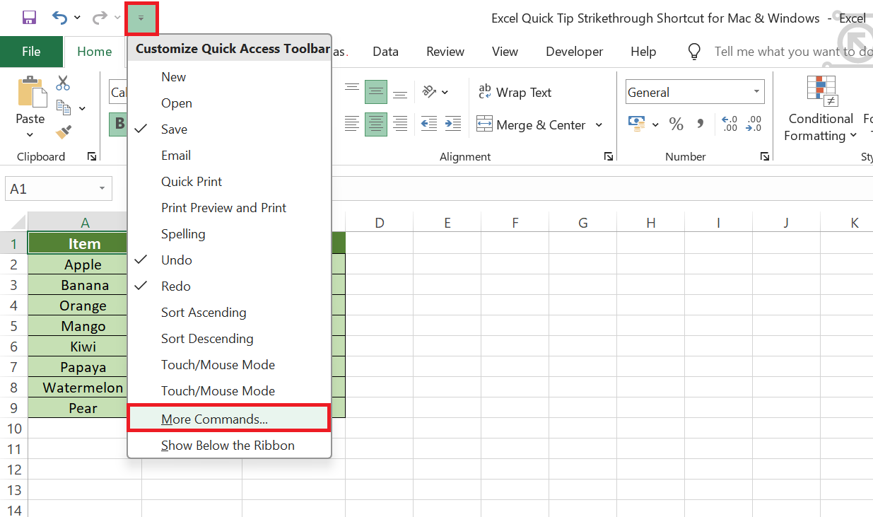
STEP 2: Expand the QAT & choose ‘More Commands…’ from the drop-down options.
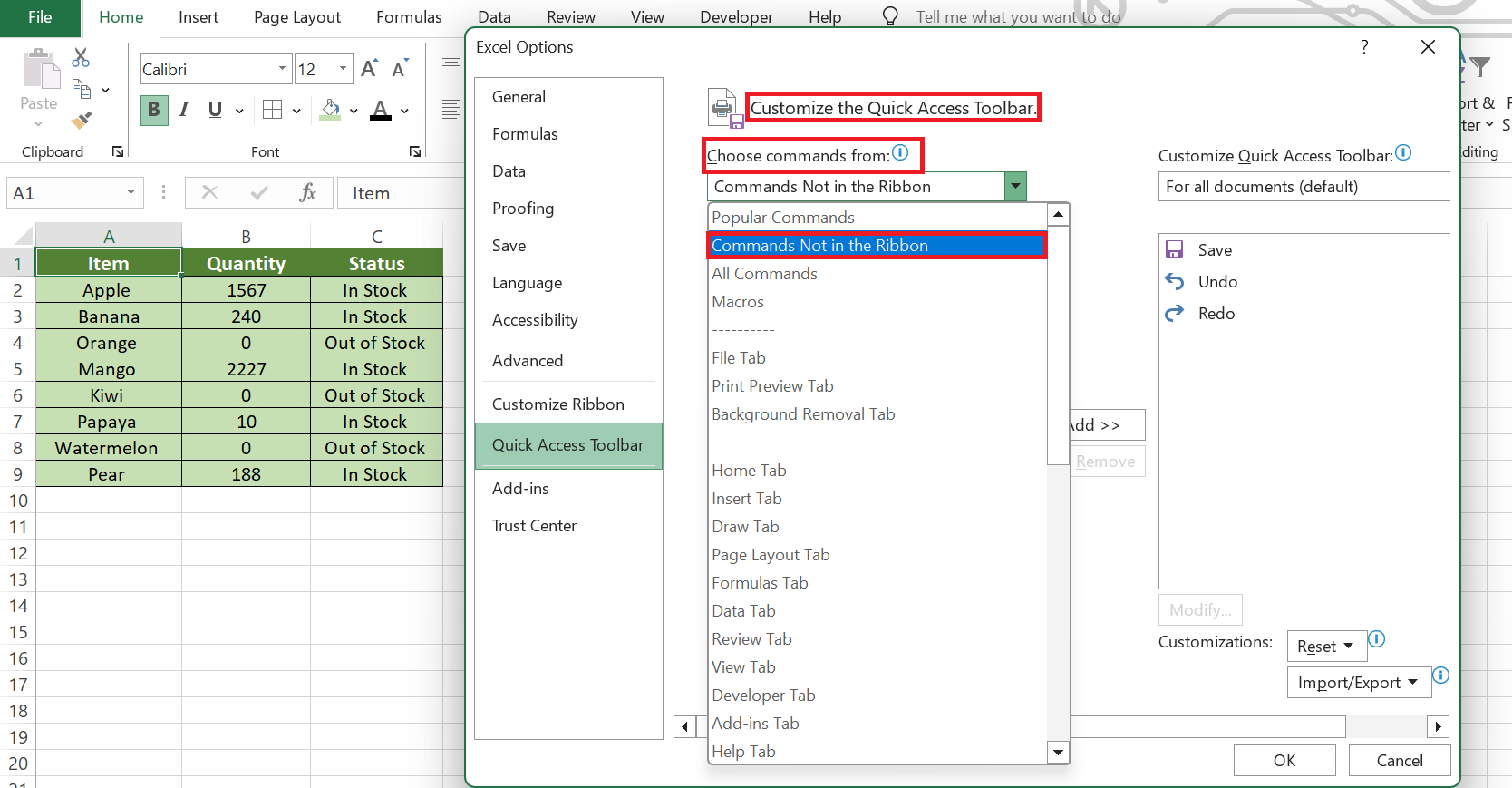
STEP 3: In the ‘Customize the Quick Access Toolbar,’ change the ‘Choose commands from:’ dropdown to ‘Commands Not in the Ribbon’.
STEP 4: Scroll down to find and select ‘Strikethrough’ then click the ‘Add >>’ button.
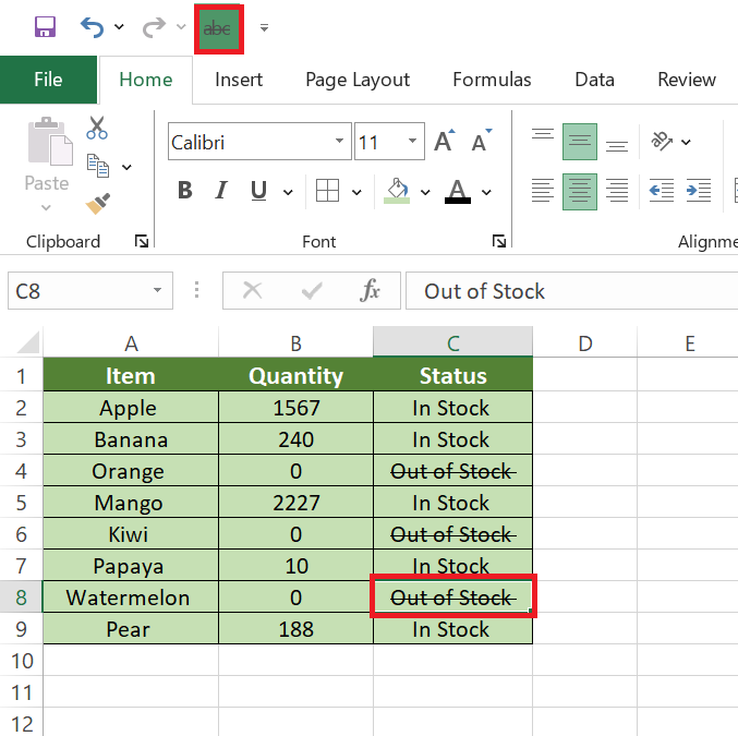
STEP 5: Hit ‘OK’ and the deed is done. The strikethrough icon now graces your QAT.
Whenever the urge strikes to strike-through, that button is ready for action, freeing you from the extra steps you’d otherwise take.
Now, the line-through effect is a single-click wonder—you could say it’s a shortcut to a shortcut, making your workflow smoother and letting you strike through the noise with speed and grace.
Essentially, by customizing your QAT, you’re crafting your very own Excel command center, tailored just for your daily tasks and efficiency.
Cross-Platform Tips for Using Strikethrough
How to Strikethrough Only Part of a Cell
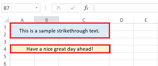
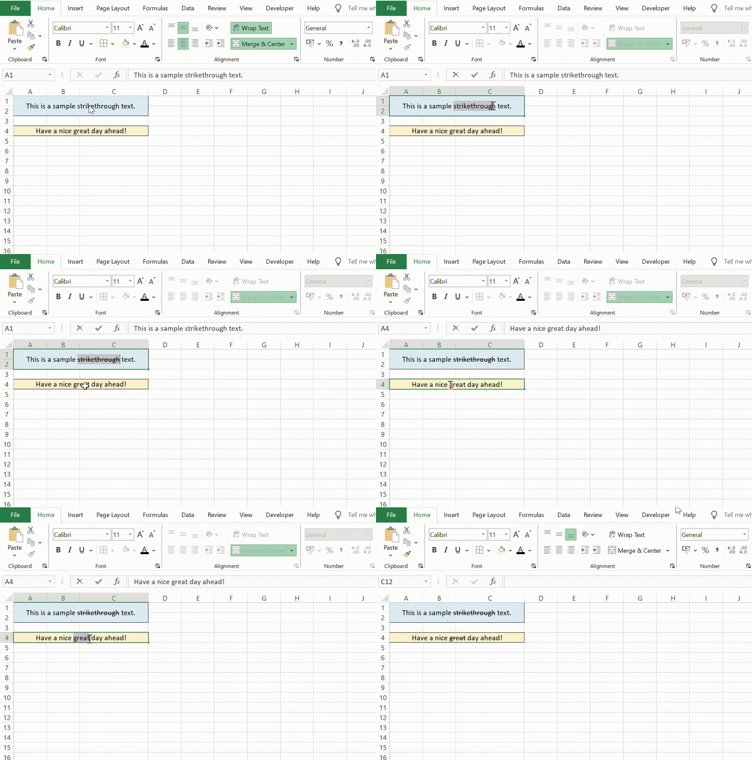
Need to make just a word or a chunk of text in a cell walk the line? It’s possible! Here’s how to apply that selective strikethrough in Excel:
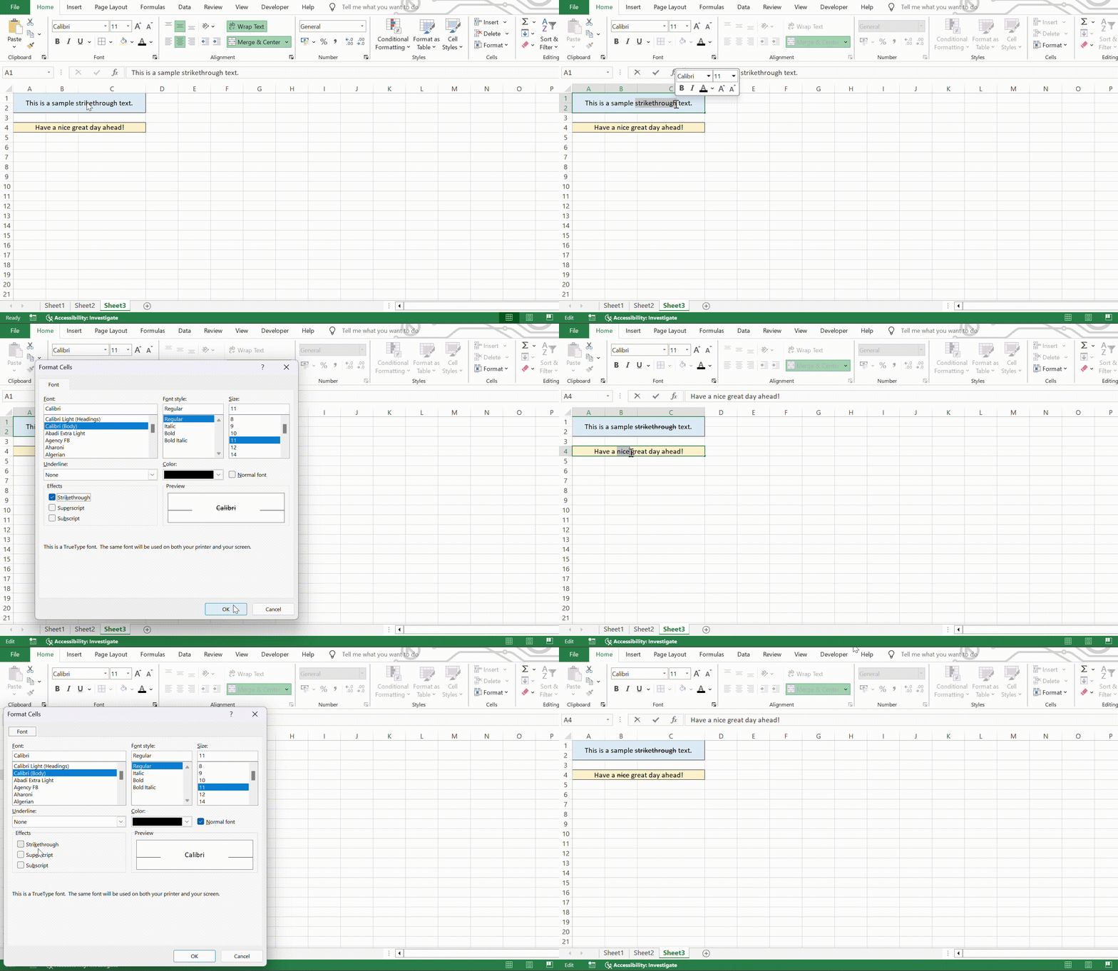
STEP 1: Input your text into Excel cells.
STEP 2: After typing, manually select the specific word or phrase you want to strike through. Right-click and choose “Format Cells.” In the Format Cells dialog box, go to the Font tab, and check the “Strikethrough” option. Click OK. Repeat step 2 for each word or phrase you want to selectively strike through in different cells or within the same cell by manually selecting them and applying the formatting.
STEP 3: Alternatively, press Ctrl + 5 (or ⌘ + Shift + X on a Mac) to apply that stylish strikethrough and boom—partial text crossed out.
This handy trick allows you to send a precise message about specific elements within a cell, keeping the rest untouched and visible.
Remember, the goal is to communicate effectively—not just about what’s complete or obsolete but also to show what still demands attention. That’s the power of partial strikethrough; it’s a nuanced paintbrush in your data visualization toolkit.
Conditional Formatting with Strikethrough for Dynamic Data Presentation
When your spreadsheet is the stage, and data’s the star, conditional formatting with strikethrough is like the director—cueing the right visual cues at precisely the right time. This feature allows cells to adapt, putting on a strikethrough costume automatically when they meet your set of rules.
Here’s the lowdown on setting the stage for conditional strikethrough:
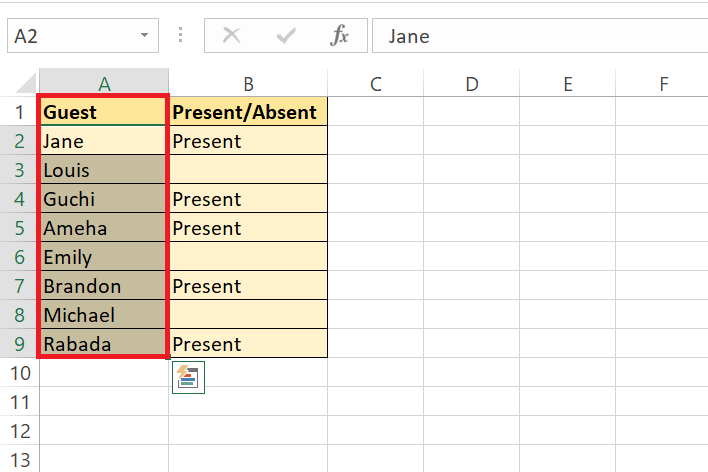
STEP 1: Highlight the cells you want the rules to apply to.
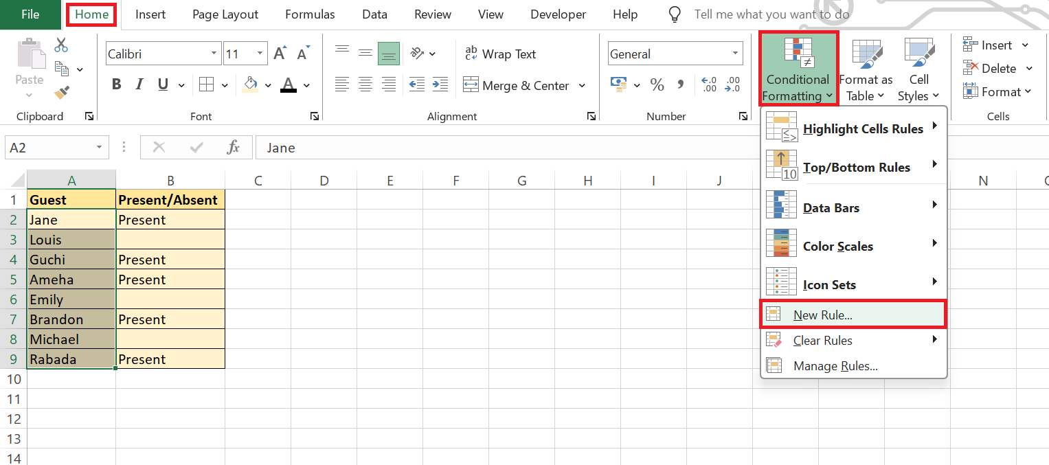
STEP 2: Dive into the ‘Home’ tab and choose ‘Conditional Formatting’, then ‘New Rule…’
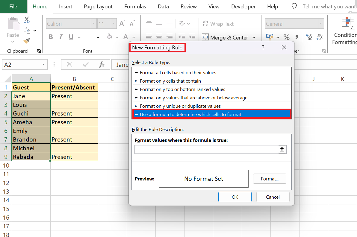
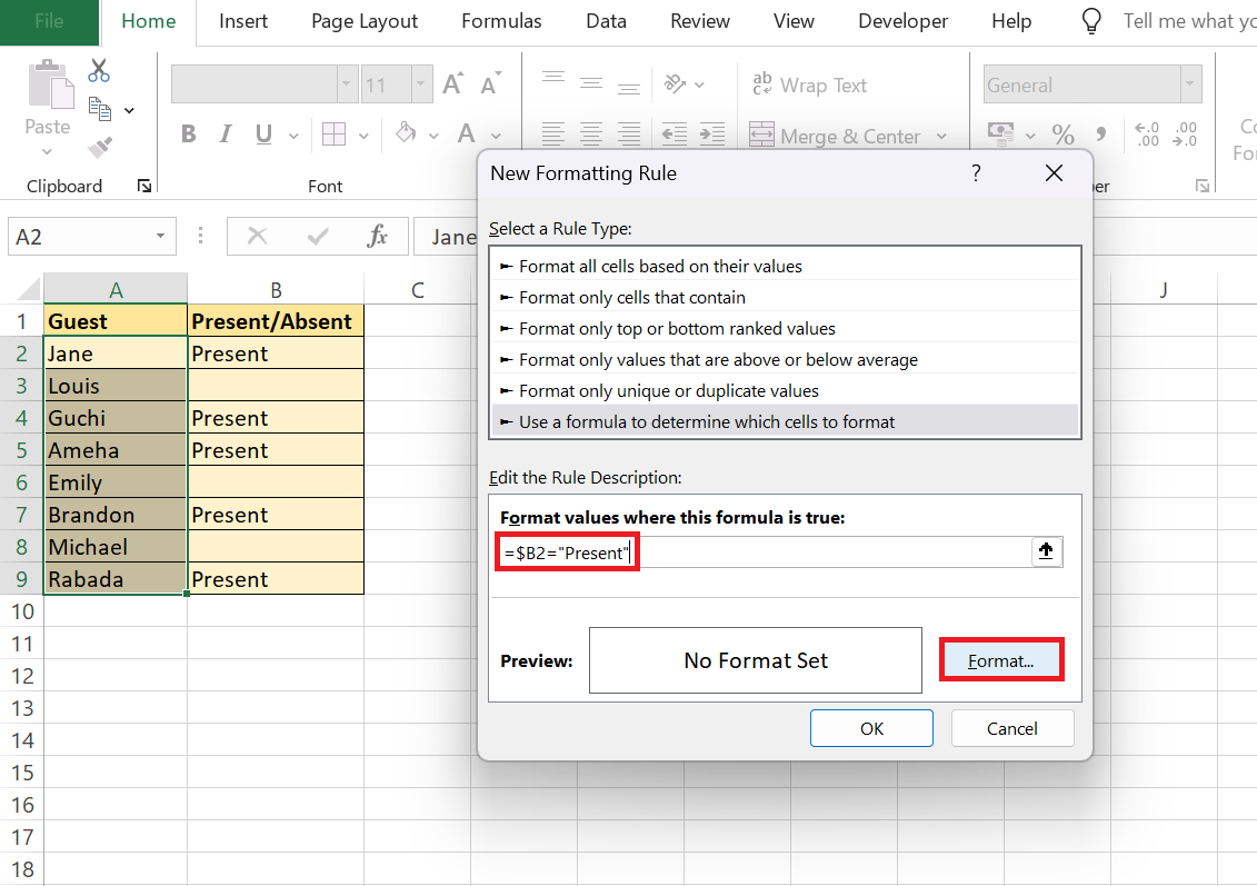
STEP 3: Opt for ‘Use a formula to determine which cells to format’.
STEP 4: Craft your formula. For instance, =$B2="Present" will hunt down cells where “Present” is written. Then hit ‘Format…’,
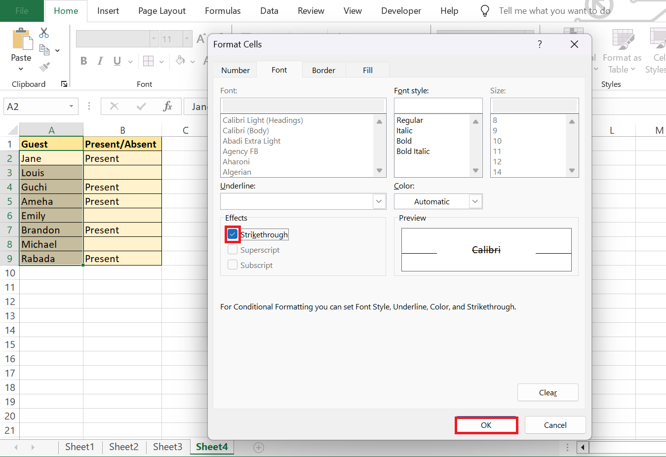
STEP 5: Flick on the ‘Strikethrough’ checkbox in the ‘Font’ tab. Click ‘Ok”
STEP 6: After clicking on ‘OK’ once more, the deal is sealed.
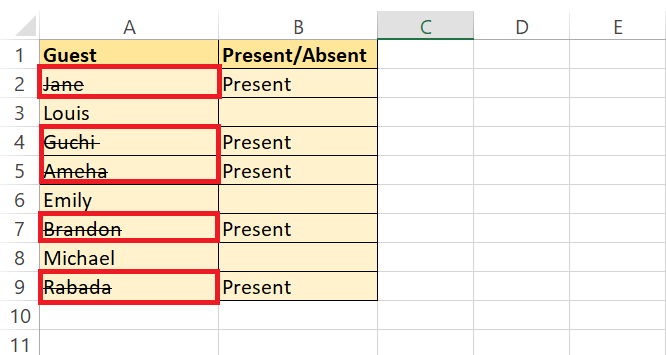
Now, like a spreadsheet chameleon, the cells will change their look—in this case, strike out text—based on your set of rules.
Conditional strikethrough adds depth to your data’s story, highlighting progress, changes, or areas that need attention without manual updates.
Immerse yourself in the freedom and clarity this brings—watching your data-style itself on the fly is a bit like having an assistant who anticipates your needs before you even vocalize them.
Whether it’s tracking project milestones or managing inventory, conditional strikethrough is a dynamically, turning your Excel canvas into an interactive dashboard.
Advanced Techniques and Troubleshooting
Utilizing Macros for Strikethrough Formatting
Embracing Macros in Excel is like having a wizard by your side. You can create a spell—or in Excel terms, a macro—to add the strikethrough format with a flourish that no muggle manual method can match. Let’s brew this enchanting potion:
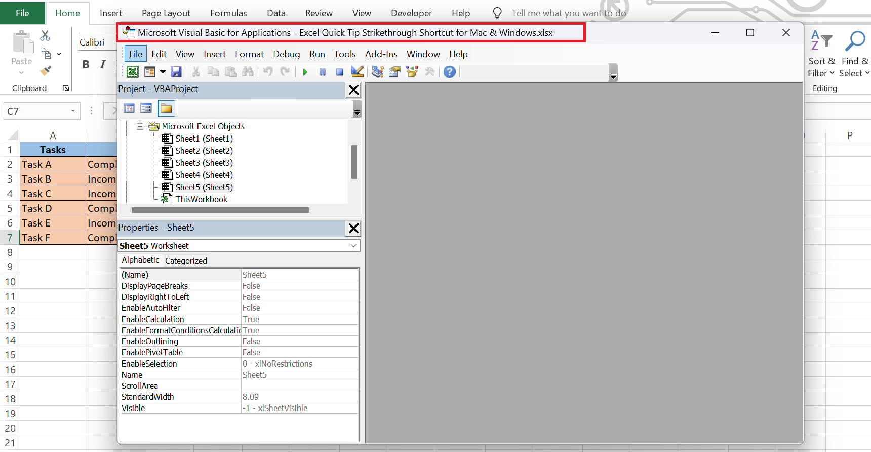
STEP 1: Invoke the VBA editor by pressing Alt + F11 when you’re in Excel.
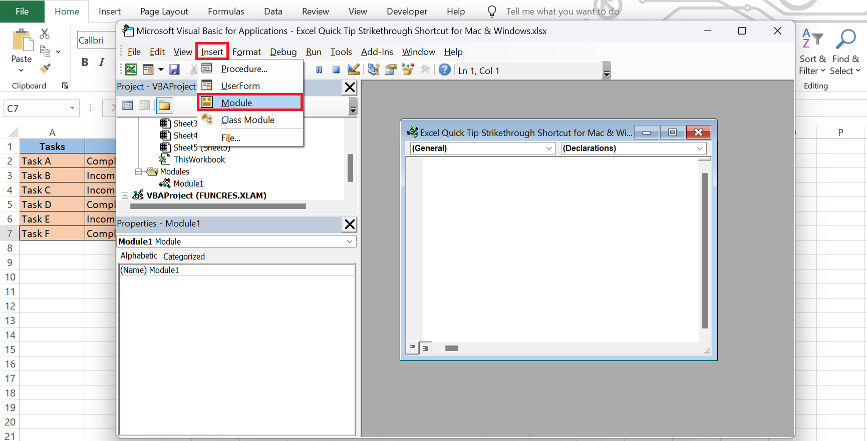
STEP 2: Click on ‘Insert’ from the menu, and select ‘Module’ to weave your new magic area.
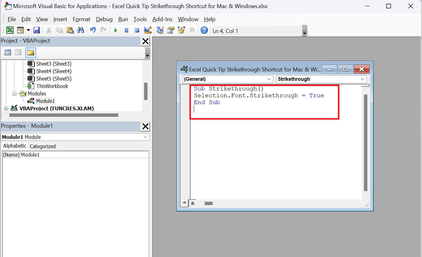
STEP 3: In the module cauldron, conjure up the following code:
Sub Strikethrough()

Selection.Font.Strikethrough = True

End Sub
Once this macro is invoked, it’ll leap into action, striking through whatever you’ve highlighted.
Remember the incantation: Macros apply their charm to the selected range. So, before you unleash the spell, make sure you’ve chosen the right cells for the transformation.
Whether you’re in the world of budgeting spells or scheduling charms, a strikethrough macro can slash your formatting time, letting you focus on the real magic: analyzing and interpreting your data’s story.
FAQ: Excel Strikethrough Shortcut Insights
Can I Split a Cell and Apply Strikethrough in Excel?
Absolutely, you can split the contents of a cell into separate cells using the ‘Text to Columns’ feature and then apply strikethrough formatting individually. Just remember, splitting cells is different from applying partial strikethrough within a single cell.
Make sure your data is prepped and ready for splitting to keep everything tidy and intentional. Once split, use your strikethrough shortcut or formatting menu to cross out what’s needed—leaving your data clearly communicated and visually on point.
How Do I Remove Strikethrough Applied by Mistake?
Oops! If strikethrough sneaks into your cell by accident, reverse it with a cinch. Press Ctrl + 5 (Windows) or ⌘ + Shift + X (Mac) with the cell selected. This toggle removes the strikethrough just as easily as it was applied.
Insert Quick Undo GIF Placeholder: Removing accidental strikethrough with keyboard shortcut
Or, dip into the ‘Format Cells’ dialog (Ctrl + 1 or ⌘ + 1), untick the strikethrough option, and say goodbye to the unwanted line-through. Your data will be back to its pristine state before you know it.
Are There Alternative Methods to Strikethrough Without Shortcuts?
Certainly! If shortcuts aren’t your cup of tea, the traditional route via the Format Cells dialog is your next best friend. Right-click the cell(s) in question, pick ‘Format Cells,’ then hop over to the Font tab, tick the strikethrough box, and hit OK.
This method can be a few more clicks, but it’s straightforward and gets the job done, especially if you’re already navigating through other formatting options. It’s also a favorite for the mouse mavens who prefer a more point-and-click approach to their Excel escapades.
Is there a shortcut for Strikethrough in Excel?
Yes, there is! To swiftly apply a strikethrough in Excel, use these keyboard shortcuts:
- On Windows, press Ctrl + 5.
- On Mac, the shortcut is ⌘ + Shift + X.
These shortcuts are quick, reliable, and work on selected text within a cell or on the cell as a whole. Jump into the fast lane of formatting with these key combinations.
How to apply strikethrough on excel mac version?
Applying strikethrough in Excel on a Mac is a breeze with this sleek shortcut:
- Press ⌘ + Shift + X after selecting the text or cell you want to format.
Alternatively, dive into the Format Cells dialog (⌘ + 1), tick the strikethrough checkbox under the Font tab, and voilà—your text is crossed out with the precision of a digital tailor.
How possible to copy/link the formatting part as well?
Copying or linking formatting—including strikethrough—in Excel is doable using the Format Painter. This handy tool clones your formatting from one cell and brushes it onto another with just a couple of clicks:
- First, click the cell with the strikethrough you’d like to copy.
- On the ‘Home’ tab, click the paintbrush icon known as the ‘Format Painter’.
- Then, paint away! Click on the cell(s) where you want the strikethrough applied.
When the paint dries, you’ll see your stripes replicated exactly where you wanted. It’s a smooth way to ensure consistent formatting without reapplying settings from scratch.
John Michaloudis is a former accountant and finance analyst at General Electric, a Microsoft MVP since 2020, an Amazon #1 bestselling author of 4 Microsoft Excel books and teacher of Microsoft Excel & Office over at his flagship MyExcelOnline Academy Online Course.

