Table of Contents
Download the Excel Workbook below to follow along and understand how to use subtraction in Excel – download excel workbookSubtraction-in-Excel.xlsx
Introduction to Subtraction in Excel
There is a no-inbuilt formula that can be used to subtract in Excel. But, we can use the minus (-) operator to subtract values and allow users to find differences between numbers, dates, time values, and even percentages.
The syntax for Subtraction in Excel is –
=Number1 – Number2
where, number1 and number2 can be numbers, cell references, dates, times, percentages, or any other mathematical expression.
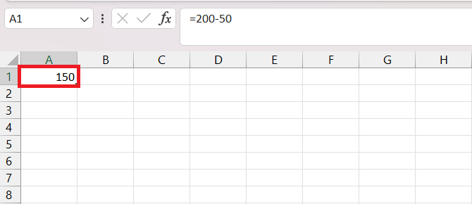
For example, we can subtract 50 from 200 by using the following steps below –
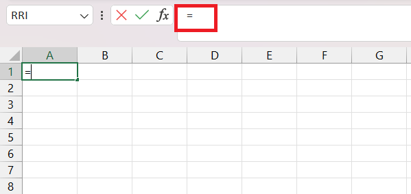
STEP 1: Enter the equal to sign (=) to begin the formula
=
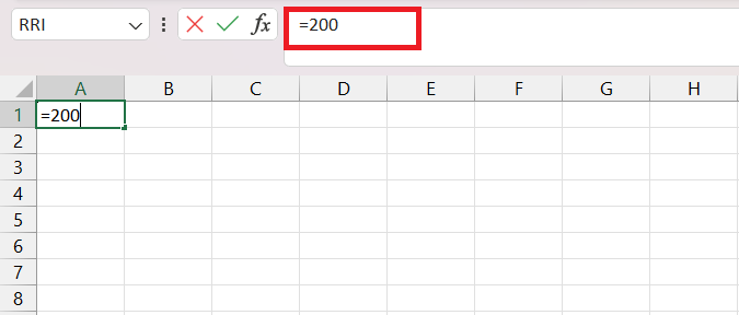
STEP 2: Enter the number from which another number is to be subtracted i.e. 200
= 200
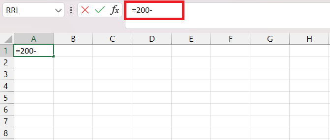
STEP 3: Enter the minus operator (-).
=200 –
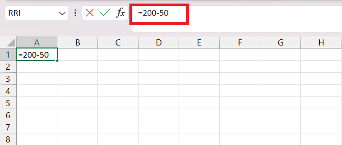
STEP 5: Enter the number to be subtracted i.e. 50.
= 200 – 50
After subtracting 50 from 200, the result i.e. 150 will be displayed.
#1 – Subtract Cells in Excel
Instead of entering the number in the formula, we can use an alternative approach of using cell references. By employing cell references, the formula becomes dynamic i.e. it can automatically update the value whenever a modification is made. This ensures flexibility, making it a preferred approach in Excel.
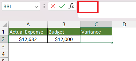
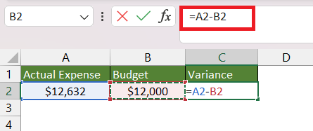
Suppose we have actual expenses in one column (Column A) and budgeted expenses in another column (Column B) and we want to calculate the variance by using subtraction in Excel. Here, we can enter the numbers in the formula directly but it can lead to human error. Also, if there is any change in numbers later we will have to manually update the formula.
So, it is advisable to use a cell reference. We can do so by following the steps below –
STEP 1: Enter the equal to sign (=) to begin the formula
=
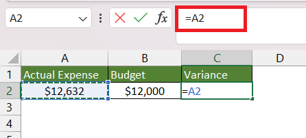
STEP 2: Enter the cell reference containing the actual expenses i.e. A2
= A2
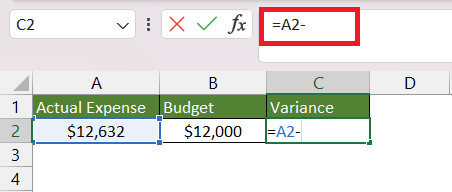
STEP 3: Enter the minus operator (-).
=A2 –
STEP 5: Enter the cell reference containing the number to be subtracted i.e. B2.
= A2 – B2
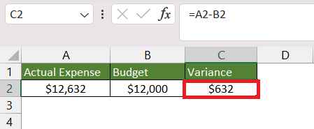
After subtracting budgeted expenses from actual expenses, the variance between the two will be displayed in cell C2.
#2 – Subtract Dates in Excel
In Microsoft Excel, dates are treated as numerical values and are internally stored as serial numbers. The date serial number system starts from January 1, 1900, which is assigned the serial number 1. Serial numbers for dates increase sequentially based on the number of days that have passed since January 1, 1900.
This is the reason why we can easily use the minus operator to subtract dates in Excel.
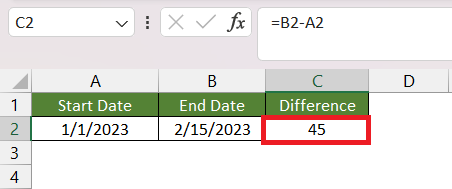
Consider the following example: in cell A2, you have the start date (i.e. 01-Jan-2023), and in cell B2, you have the end date (i.e. 15-Feb-2023). To find the number of days between the two dates, you can use the formula:
= B2 – A2
Excel will automatically calculate the difference and display the result (45 days) in cell C2.
#3 – Subtract Time in Excel
To subtract time in Excel, we can use the minus operator (-) just like we would with numbers and dates.
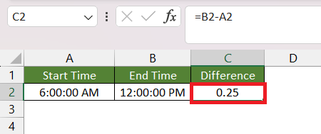
Consider the following example: in cell A2, you have the start time (i.e. 6 AM), and in cell B2, you have the end time (i.e. 12 PM). To find the time difference, you can use the formula:
= B2 – A2
Excel will automatically calculate the difference and display the result (i.e. 0.25) in cell C1.
In Excel, time is depicted in decimal format. For instance, 0.5 corresponds to 12 hours, indicating it represents half of a day. So, in this example, 0.25 corresponds to 6 hours i.e. a quarter of a day.
#4 – Subtract Percentages in Excel
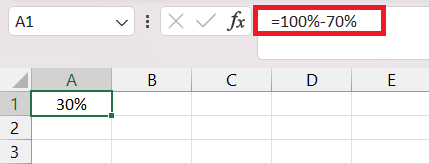
When we need to subtract one percentage from another, we can easily achieve it using the familiar minus formula. For example:
=100% – 30%
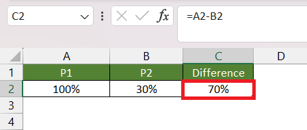
Alternatively, if you prefer entering the percentages in separate cells, you can use cell references to subtract them like this:
=A2 – B2
Both methods are effective in Excel and allow you to perform percentage calculations effortlessly.
#5 – Subtract same number from range of numbers
When working with a range of numbers, you might find a need to subtract a specific number from each cell in the column. While we can use manual calculations and subtract them individually from each cell, Excel’s “Paste Special” feature provides a quick and efficient way to accomplish this task.
To subtract one number from a column of numbers using Paste Special in Excel, follow these steps:
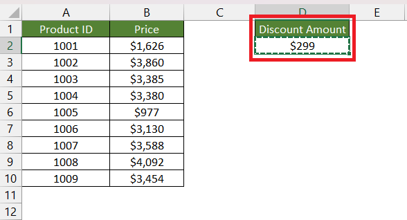
STEP 1: Copy the number you want to subtract. Here, it is 299 entered in cell D2.
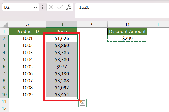
STEP 2: Select the range of cells that you want to subtract from. Here, it is B2:B10.
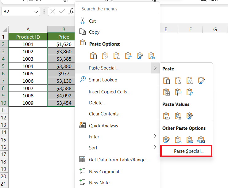
STEP 3: Right-click on the selected range of cells and choose Paste Special.
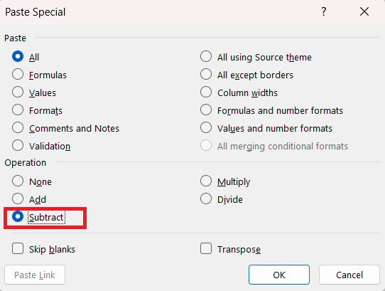
STEP 4: In the Paste Special dialog box, choose Subtract. Click OK.
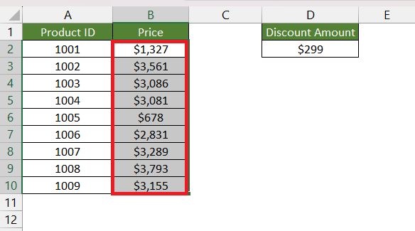
Excel will subtract the number you copied (i.e. 299 ) from each cell in the selected range and display the result.
Conclusion
Subtraction in Excel is one of the basic arithmetic operations that can be used to find differences between numbers, dates, time values, and percentages. Users can either directly subtract values or use cell references to create dynamic formulas for automated updates.
Excel also offers the Paste Special feature to quickly subtract the same number from a range of numbers in a column.
Click here to learn more about how to use subtraction in Excel.
John Michaloudis is a former accountant and finance analyst at General Electric, a Microsoft MVP since 2020, an Amazon #1 bestselling author of 4 Microsoft Excel books and teacher of Microsoft Excel & Office over at his flagship MyExcelOnline Academy Online Course.

