Top 5 Ways to Sum a Row in Excel

In the fast-paced realm of business, efficiency is paramount. Microsoft Excel emerges as a critical ally, enabling professionals to execute rapid calculations with unwavering accuracy. Summing a row, a seemingly simple task epitomizes the essence of quick and precise decision-making based on thorough data analysis.

Introduction to Mastering Row Summation in Excel

The Significance of Quick Calculations

In today’s fast-paced business environment, efficiency isn’t just an advantage—it’s a necessity. Excel, a powerful tool in the arsenal of any professional, stands at the ready to crunch numbers at lightning speed. Precision and speed in Excel are not just about saving time; they’re about making accurate decisions based on solid data analysis. That’s where quick calculations, like summing a row, become essential.

Overview of Row Summation Techniques

Summing rows in Excel is a common task, one you might encounter while working with financial statements, inventories, or any dataset requiring quick total calculations across a horizontal array of numbers. There are various techniques available in Excel to perform these sums:

• Manual Addition: Add cell references individually using the plus (+) operator.
• SUM Function: Utilize the SUM() function for a cleaner and more efficient approach.
• AutoSum Feature: Click the AutoSum button (Σ) to sum a row or column instantly.
• Excel Tables with Total Row: Activate the total row in an Excel table to auto-calculate sums for each column.
• Conditional SUM: Use the SUMIF() function with Excel.

Whether you’re a beginner or an Excel enthusiast, understanding these techniques will equip you with the flexibility to choose the best method based on your specific task.

 

Step-by-Step Guide to Sum a Row

Method 1: Using Basic Arithmetic for Row Addition

When you’ve got just a handful of cells to sum, basic arithmetic within Excel can come to the rescue. Simply use the plus sign (+) operator to add up the values, just as you would in a regular math calculation. Here’s how you step up your game:

STEP 1: Click on the cell where you want the total sum to appear.

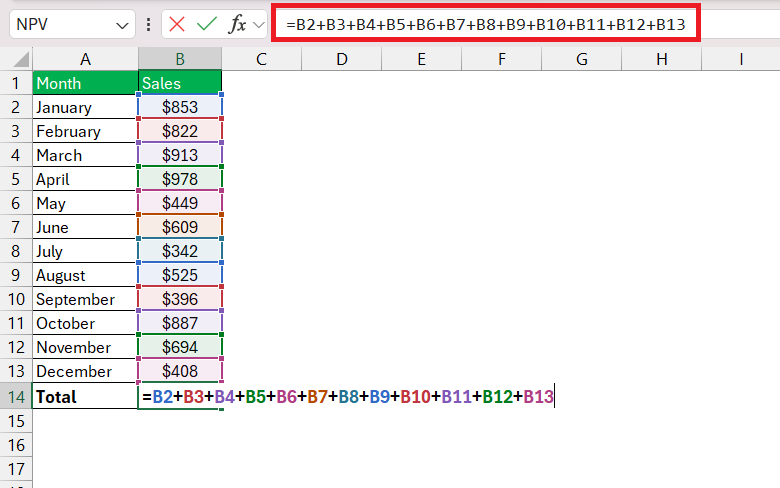
STEP 2: Type in = followed by the cell references you wish to add, separating each with a +. For example, a sum of cells from B2 to B13 would look like =B2+B3+B4+B5+B6+B7+B8+B9+B10+B11+B12+B13.

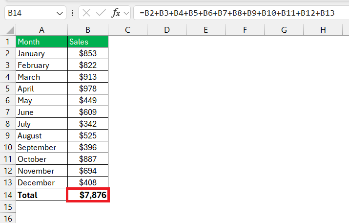
STEP 3: Then hit Enter, and voilà, the sum appears!

Although this method is straightforward, it’s best suited for scenarios with fewer cells. When dealing with a large number of cells, it can become cumbersome and error-prone.

 

Method 2: Harnessing the Power of Excel’s SUM Function

When it comes to adding up a longer row of numbers with ease and avoiding the potential pitfalls of manual entry, turning to Excel’s SUM function is your best bet. This function is designed specifically for totaling numbers, and you’ll find it indispensable for larger datasets.

The SUM function is like a Swiss Army knife for number crunching in Excel. It’s deceivingly simple yet incredibly versatile, allowing you to effortlessly tally up numbers in a row—or any range for that matter—with a straightforward formula: SUM(number1, [number2],...).

The first number is required, while those in square brackets are optional.

Here’s how to utilize it for summing a row:

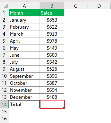
STEP 1: Click the cell where you want to see the row’s total.

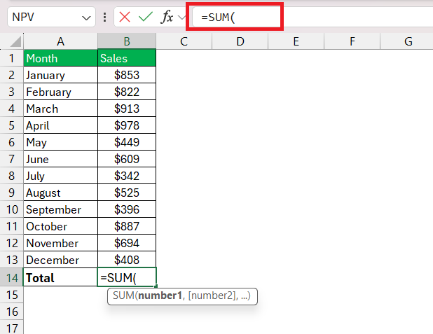
STEP 2: Enter the SUM function followed by an open parenthesis.

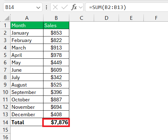
STEP 3: Highlight the row of cells you wish to sum or type the range manually, like SUM(B2:B13). Close the parenthesis and press Enter.

This swift method ensures accurate results and is tailored for times when you need to sum a row quickly and reliably. It’s also dynamic – if you add or change the figures in the referenced cells, the sum updates automatically, making it easier to maintain data over time.

 

Method 3: AutoSum Magic: Adding Large Rows Instantly

The AutoSum feature, as hinted previously, is like a flash of lightning in summing large rows of data. This Excel trick is perfect when you’re looking at rows brimming with numbers and you need a total, fast. It works like this:

STEP 1: Click on the cell at the end of the row where you want the grand total to shine.

STEP 2: Press the AutoSum button (Σ) on the Home tab, or for more flair, use the ALT + = shortcut. Excel, grasping your need for speed, automatically selects the adjoining row of numbers.

STEP 3: Now comes the encore: press Enter and watch the sum appear with almost no effort.

For those frequent tasks involving large data sets or when you’re flipping between tasks, AutoSum’s speedy service lets you focus on what the numbers are telling you, rather than the process of adding them up.

This feature shines when you’re working with long columns or rows and want a sum total in record time, without the fuss of manual data selection.

• Effortless to use: Position the cursor, click the button, and presto—calculation complete!
• Saves time: Instantly adds up numbers without manually typing formulas.
• Avoids errors: Reduces the chance of selecting the wrong range when summing.
• Versatile: Works with columns and rows alike.
• Smart detection: AutoSum identifies adjacent numerical data for quick results.

However, remember that AutoSum relies on nearby data, so if your data isn’t contiguous, you may need to select the range manually.

Remember, AutoSum is adaptable; it’s your go-to whether you’re summing up rows or columns. It’s smart, snappy, and smooth, turning what could be minutes into mere moments.

 

Method 4: Excel Tables with Total Row: The Organized Approach

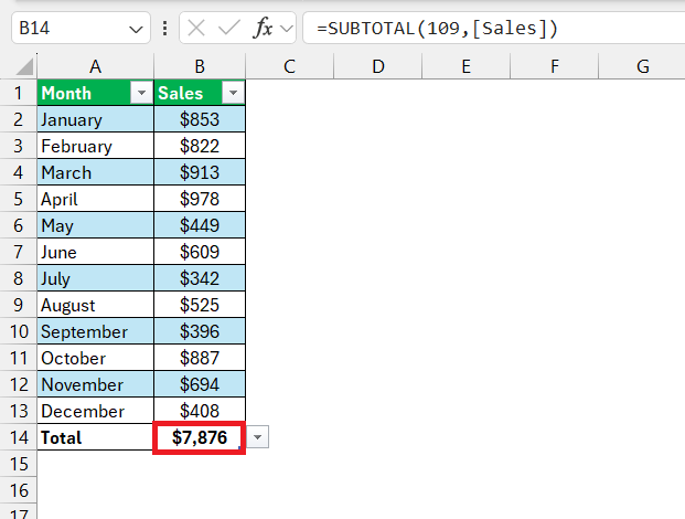
Excel tables offer a structured and feature-rich way to manage data. By converting a range of data into a table, users can easily activate a total row, which provides automatic calculations for each column, including sums.

To activate the total row, simply check the Total Row option under the Table Tools Design tab.

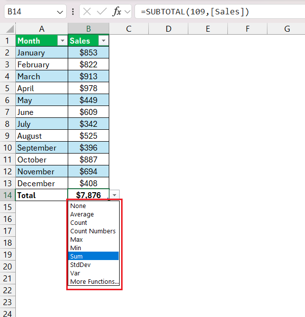
This method not only sums your data but also enhances data organization and provides easy access to a suite of other calculations. You can even change the operation from SUM to COUNT, AVERAGE, MINIMUM, etc.

Method 5: Efficient Data Handling with SUMIFS for Multiple Criteria

The SUMIFS function elevates the art of summing in Excel by enabling you to include specific conditions or multiple criteria. It’s particularly useful when you want to sum a row based on certain parameters—like sales in a particular region or within a certain date range. Here’s a brief guide on how to work with SUMIFS:

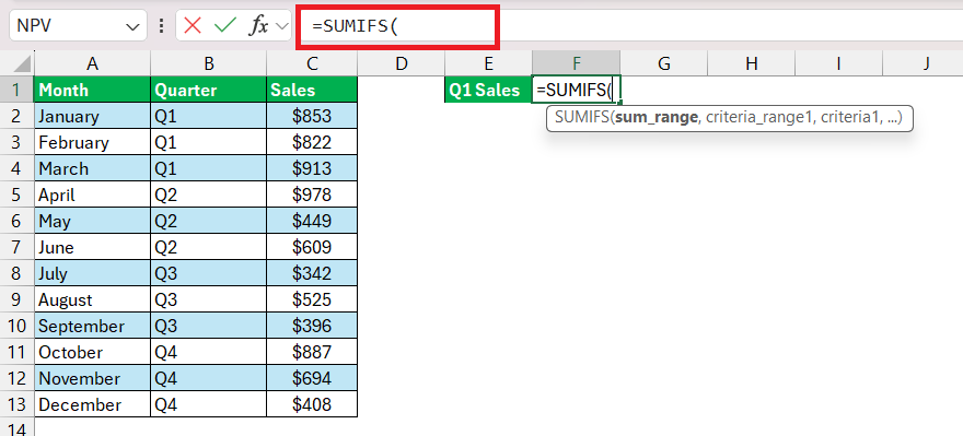
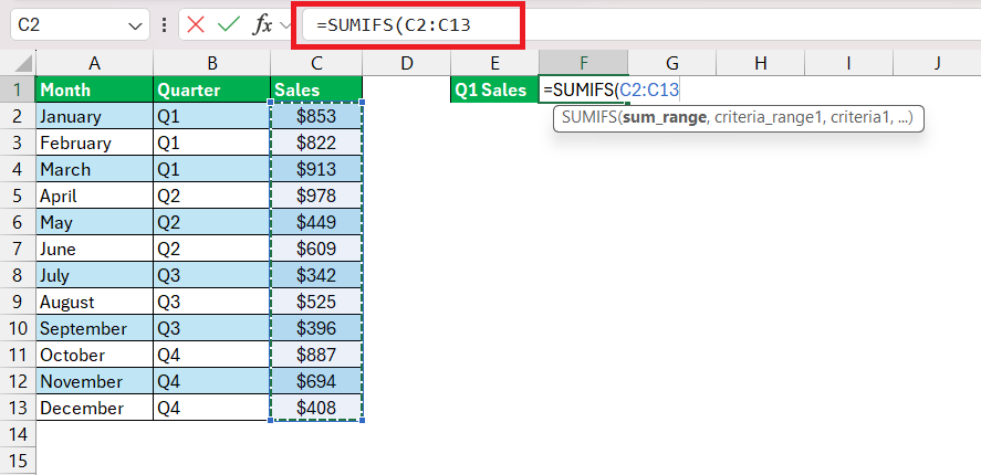
STEP 1: Open the cell where the conditional total will be displayed. Type =SUMIFS( to start your function.

STEP 2: The first argument is your sum_range, the actual cells you’re adding up.

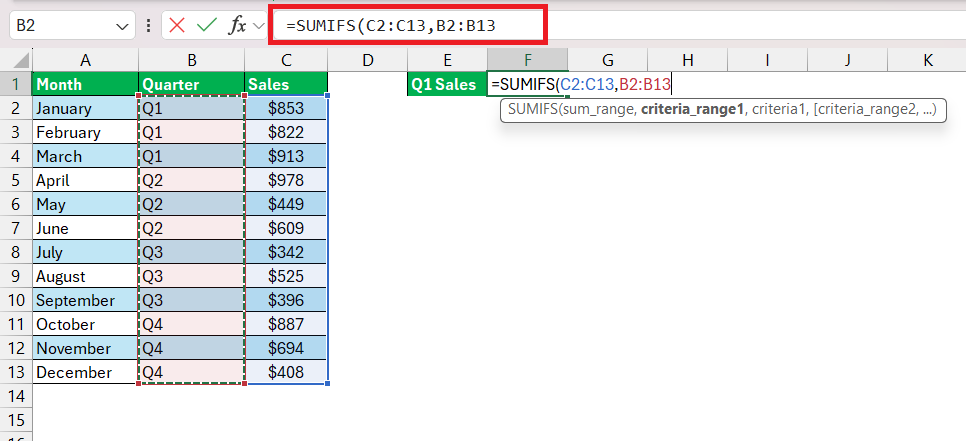
STEP 3: Next, define criteria_range1 which is the range to check for your first condition.

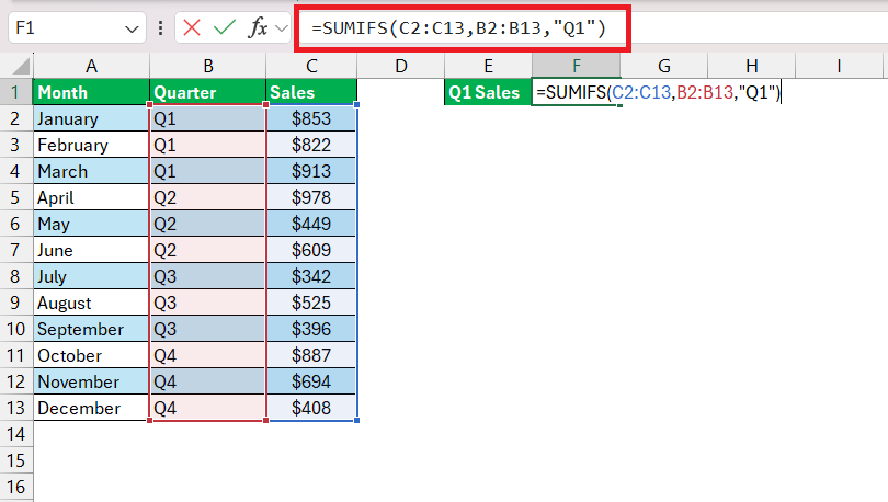
STEP 4: Specify your criteria1, the condition that must be met.

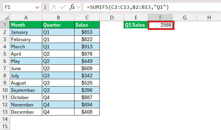
STEP 5: Once all your ranges and criteria are in place, close it off with a parenthesis and press Enter.

This formula would sum all values in cells C2 through C13 where the corresponding cells in B2 through B13 are “Q1”.

If needed, continue adding conditions by entering additional criteria_range and criteria pairs.

The SUMIFS function can be a game-changer, offering you the ability to analyze and sum data precisely. Its multi-criteria capacity ensures data is not just totaled, but intelligently totaled based on your targeted conditions.

 

Conclusion

Summing a row in Excel is a foundational skill that ranges from basic manual addition to advanced functions like SUMIFS. Each method serves its purpose, from quick calculations with AutoSum to detailed analysis with SUMIFS. Understanding these techniques equips you with the flexibility to tackle any summing task, ensuring efficiency and accuracy in your Excel endeavors.

Whether you’re a beginner or an Excel veteran, these tips will enhance your data management skills, allowing you to sum a row like a pro in seconds.

 

Frequently Asked Questions

How do I sum an entire row in Excel?

To sum an entire row in Excel, use the SUM function with a full row reference like this: =SUM(5:5). This will sum all values in the 5th row. As you add more data to the row, the sum will automatically update to include the new values.

How do I sum a row in a table in Excel?

In an Excel table, click the cell at the end of the row you want to sum. Then, either use the AutoSum feature by pressing ALT + = or enter the SUM function manually, like =SUM(Table1[@[Column1]:[Column5]]), to sum a specific row within a table.

How can I sum a row that includes non-numeric data?

When summing a row with non-numeric data, the SUM function will ignore text and only add up the numbers. Just type =SUM(row_range), replacing “row_range” with your row reference, and Excel will compute the total of numeric cells only.

What should I do if my row sum isn’t updating automatically?

Ensure your formula range includes the entire row, or use =SUM(5:5) for the whole row. If cells are formatted as text or there’s an error, select the problematic cells, click the warning sign, and choose ‘Convert to Number. If using dynamic arrays, use OFFSET to adjust the range.

How do you sum across rows?

To sum across multiple rows, use the SUM function with a range that encompasses all desired rows, like =SUM(B2:E2, B3:E3) to sum the first two rows in columns B through E. Alternatively, use AutoSum or drag the formula across cells.

How do I sum just visible cells?

To sum only visible cells in Excel, especially when dealing with filters, use the SUBTOTAL function with function_num as 109. The formula will look like =SUBTOTAL(109, range), which sums non-hidden rows in the specified range.