A Quick Guide to Using the SUMIF in Excel – 2 Helpful Examples

Excel, a widely-used spreadsheet software, offers a multitude of powerful features for managing and analyzing data. One such feature that proves to be extremely useful is SUMIF. The SUMIF in Excel enables you to sum values in a range that satisfies a condition.

Key Takeaways:

• The SUMIF function in Excel is an essential tool for finance professionals, enabling the quick summarization of data based on specific criteria, which can significantly enhance efficiency in performing tasks such as portfolio performance analysis and risk assessment.
• Learning to use SUMIF allows for targeted calculations, helping users to quickly isolate and aggregate numerical data that meets designated conditions—such as summing investment returns in a particular sector or during a specific time period.
• Mastery of the SUMIF function can be further leveraged by combining it with other Excel features like conditional formatting for visual data representation or integrating it into macros for automating repetitive tasks, thus expanding its utility in investment banking analytics.

Download the Excel Workbook below to follow along and understand how to use SUMIF in Excel –
download excel workbookSUMIF-in-Excel.xlsx

 

Introduction to SUMIF in Excel

SUMIF is a wisely used Excel function that allows you to sum the values in a range that meets the criteria that you specify.

SUMIF in Excel is a flexible function that may be applied in a wide range of situations, from determining sales numbers for particular goods or geographical areas to examining client information based on demographics or purchase patterns.

So if you have a list of product IDs in one column and their Sales in another column and want to Sum the sales of only one of the product IDs, then the SUMIF function is the one for you.

 

SYNTAX of SUMIF

=SUMIF(Range, Criteria, [Sum_Range])

• Range – The range that is tested using criteria. Once items in the range are found, their corresponding values in sum_range are added. Required.
• Criteria – The criteria that define which cells in the range will be added. For example, criteria can be entered as 32, “>32”, B4, “apples”, or “32”. Required.
• [Sum_Range] – The range of cells to sum. Optional.

Let us look at an example to help us understand this function better.

 

Example of SUMIF function in Excel

Example 1

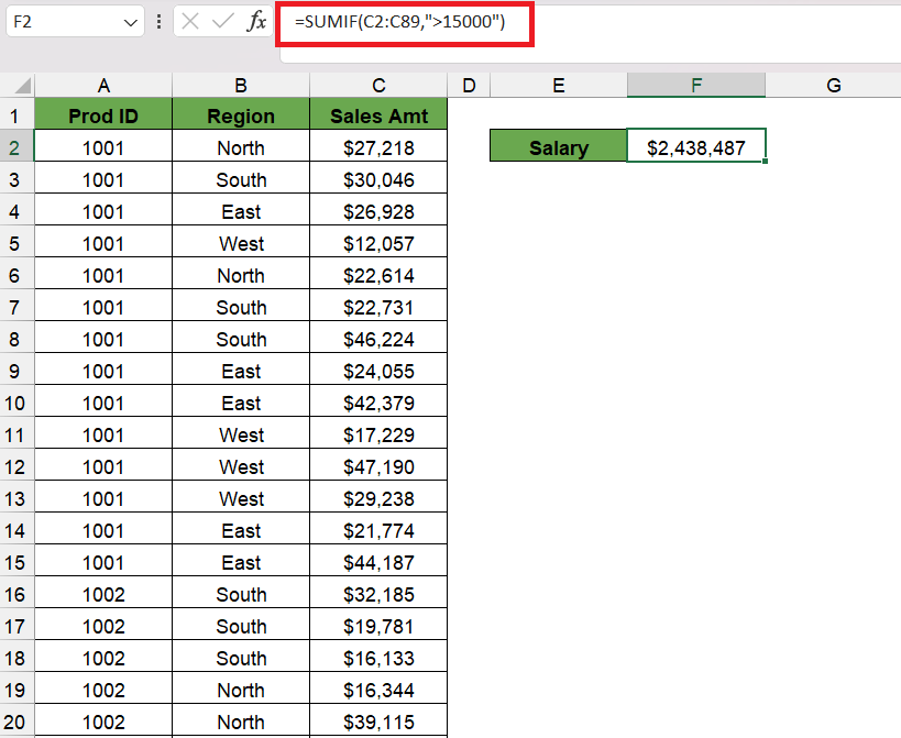
In his example, we want to get the sum of the sales amounts that are above $15,000. Follow the step-by-step tutorial below –

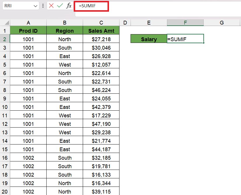
STEP 1: Enter the SUMIF function in cell F3.

=SUMIF

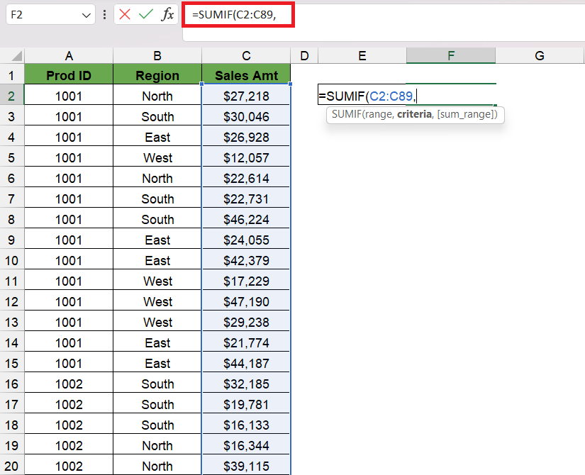
STEP 2: Enter the first argument – range. Here we have selected the range C2:C89 as it contains all the sales amount.

=SUMIF(C2:C89,

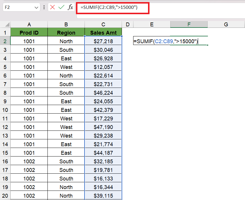
STEP 3: Enter the second argument – criteria. Here we have entered “>15000” as we want to get the sum of sales where the sales amount is greater than $15,000.

=SUMIF(C2:C89,”>15000″,

Below we can see, the SUMIF function returns the sum of sales where the sales amount is greater than $15,000.

 

Example 2

Here, we will be using the optional argument – sum_range as well. The sum_range argument is used when you want to sum values from a different range than the one used for the criteria. If your criteria are based on one column, but you want to sum values from a different column, you would use the sum_range argument.

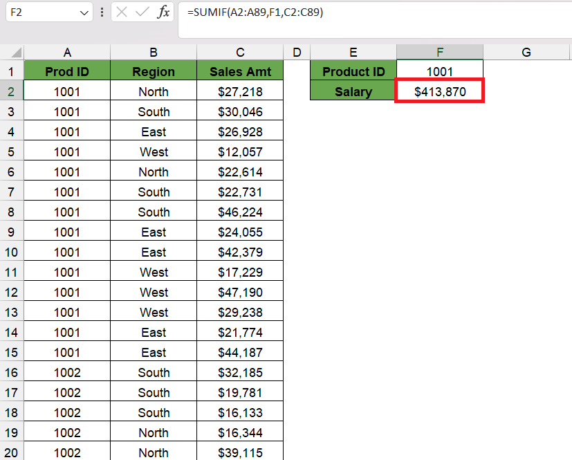
For example, if you have a list of products in column A and their corresponding sales amounts in column C, and you want to sum the sales amounts for a specific product (Product ID – 1001), you would use the sum_range argument to specify column C as the range to sum from.

Follow the step-by-step tutorial below –

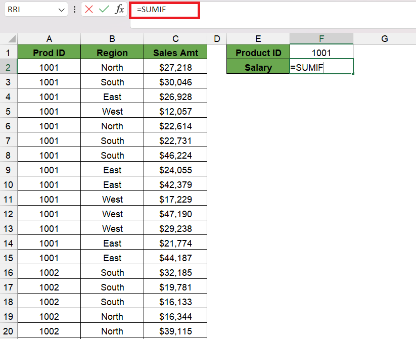
STEP 1: Enter the SUMIF function in cell F3.

=SUMIF

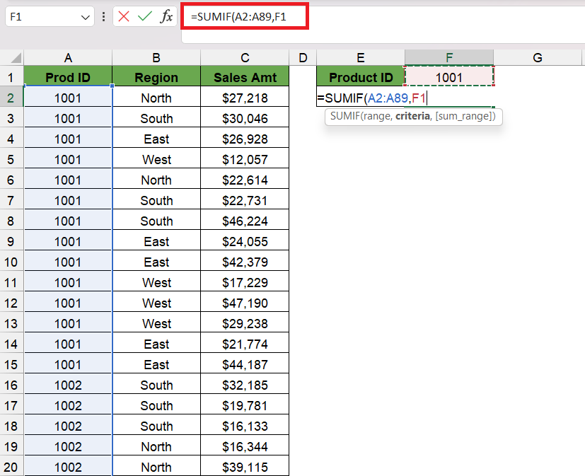
STEP 2: Enter the first argument – range. Here we have selected the range A2:A89 as it contains all the product IDs.

=SUMIF(A2:A89,

STEP 3: Enter the second argument – criteria. Here we have entered “1001” as we want the sum of sales for product ID 1001.

=SUMIF(A2:A89,”1001″,

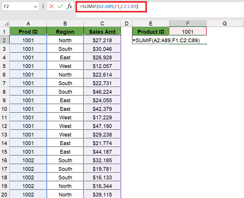
STEP 4: Enter the third argument – sum_range. Here we have selected the C2:C89 range as it contains all the sales amount.

=SUMIF(A2:A89,”1001″,C2:C89)

The SUMIF function calculates and provides the sum of sales for product 1001.

 

Restrictions of using SUMIF

Even though the SUMIF function is extremely useful, it has some restrictions that you should be aware of:

• Range size: The SUMIF function may not be appropriate for some complicated data analysis scenarios since it can become slow or cumbersome when employed with very big data sets.
• Syntax difficulty: Using the SUMIF function might be challenging, especially if you’re juggling intricate data sets. To utilize it properly, one must have a thorough understanding of Excel’s features and syntax.
• The size of each range must be uniform. A #VALUE error will be returned if the supplied ranges don’t match.
• All range arguments must be actual ranges; an array cannot be used with the SUMIF function.
• SUMIF is not case-sensitive.

Common Pitfalls and Best Practices

Debugging Common SUMIF Errors

Encountering errors when using SUMIF can be frustrating, but fear not—with a few troubleshooting tips, you can pinpoint and resolve issues quickly, ensuring your data analysis remains on track. The #VALUE! and #NAME? errors are among the most common mistakes users face.

When you see a #VALUE! error, it usually means there’s a non-numeric value where Excel expects a number, or there’s some issue with the formatting of your data. To rectify this, comb through your criteria and sum range for any anomalies, making sure all the values are formatted correctly. It’s essential to keep your criteria consistent and intentional, especially if you’re looking for numerical matches.

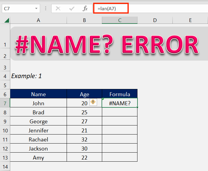
On the other hand, a #NAME? error suggests Excel doesn’t recognize a function or named range you’ve entered in your formula. This could be as simple as a typo, so check your spelling first. If you’re using named ranges, ensure that the range is defined and that you’ve referenced it correctly in your formula.

Ensuring Accuracy with Proper Formula Usage

Accuracy is paramount in data analysis to make sound decisions. When it comes to the proper usage of the SUMIF formula, a few key habits can ensure your results are always reliable.

Firstly, double-check your criteria for any non-visible characters or accidental spaces, as these can skew your results considerably. It’s especially crucial when dealing with imported data where such issues are common. Use Excel’s TRIM function to clean up your text data before applying SUMIF.

Additionally, ensure your sum range corresponds precisely to your criteria range. A mismatch, even by one cell, can shift all your results, leading to potentially misleading conclusions. Also, when referring to ranges, absolute references (using the $ sign) can safeguard against accidental changes if you copy or move the formula.

 

Frequently Asked Questions (FAQs)

Can SUMIF sum cell values based on partial text match?

Yes, the SUMIF function can sum cell values based on partial text matches. By using wildcards like the asterisk (*) for multiple unknown characters or the question mark (?) for a single character, you can create criteria for partial matches. For instance, =SUMIF(A1:A10, "*east*", B1:B10) will sum all values in B1:B10 where corresponding cells in A1:A10 contain the substring “east”. This feature is handy when dealing with variations in text data.

How do you use Sumif in Excel?

To use SUMIF in Excel, you apply the function with the following syntax: =SUMIF(range, criteria, [sum_range]). First, select your range of cells to evaluate against your criteria. Then, specify the criteria for which cells you wish to sum. If the sum range is omitted, the same range as the criteria range is summed. With this simple setup, you can quickly sum values based on specific conditions, streamlining your data analysis process.

How do I use SUMIF to sum across multiple tabs?

To use SUMIF across multiple tabs, you’ll need to repeat the SUMIF function for each tab and then add the results together. This might look like =SUMIF(Sheet1!A:A, "Criteria", Sheet1!B:B) + SUMIF(Sheet2!A:A, "Criteria", Sheet2!B:B) + SUMIF(Sheet3!A:A, "Criteria", Sheet3!B:B) and so on. There’s no direct way to do this with a single SUMIF function due to its limitations, so for multiple criteria or conditions, consider using SUMIFS with helper columns or a macro for more complex tasks.

The article introduces the SUMIF function in Excel, which is used to sum values in a range based on specific criteria. It explains the syntax of the function, consisting of the range, criteria, and optional sum_range arguments. It also provides two examples demonstrating how to use SUMIF in Excel. It also highlights some restrictions on using this function.