How to Transpose in Excel – 3 Useful Methods

Transposing data refers to rearranging the orientation of your data i.e. switching the rows to columns and vice versa. This can be a handy tool for reorganizing information to better suit your analysis, reporting, or presentation needs.

Let us look at each of these methods.

Download the Excel Workbook below to follow along and understand How to Transpose in Excel –
download excel workbookTranspose-in-Excel.xlsx

 

Method 1 – Paste Special

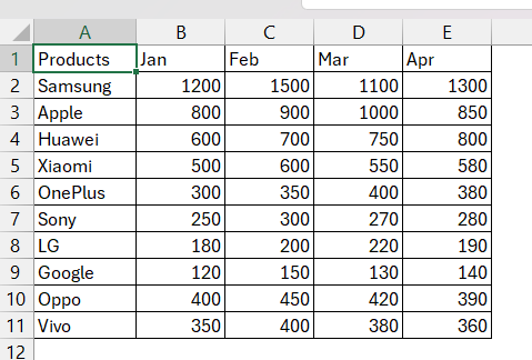
You can easily transpose data in Excel using the “Paste Special” option. Below is the sales data where –

• The rows represent different smartphones (Apple, Samsung, OnePlus, Google).
• The columns represent different months (January, February, March).

Now, you want to reverse this i.e. you want rows to represent months and columns to represent smartphones. Follow the steps below to learn how to transpose and convert rows to columns and columns to rows –

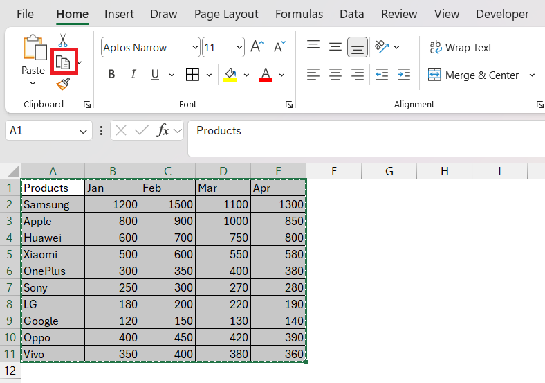
STEP 1: Highlight the sales data table and go to Home > Copy.

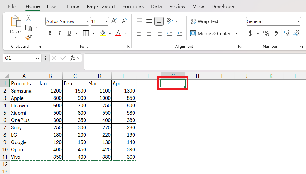
STEP 2: Move to the cell where you intend to place the transposed data.

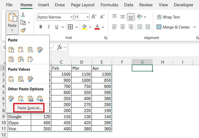
STEP 3: Go to Home > Paste > Paste Special.

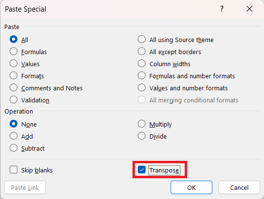
STEP 4: In the Paste Special dialog box, select Transpose and Click OK.

The transposed data will now be pasted in cell G1.

This method is quick and easy but is best suited for smaller datasets. It is useful when you do not want the transposed data to be linked to the original data.

Method 2 – TRANSPOSE Function

In the previous method, the transposed data remains static i.e. any change you make in the original data will not affect the transposed data. If you use the TRANSPOSE function you can link the original data with the transposed data.

Follow the steps below to learn how to use the TRANSPOSE function in Excel –

STEP 1: Go to the cell where you intend to place the transposed data.

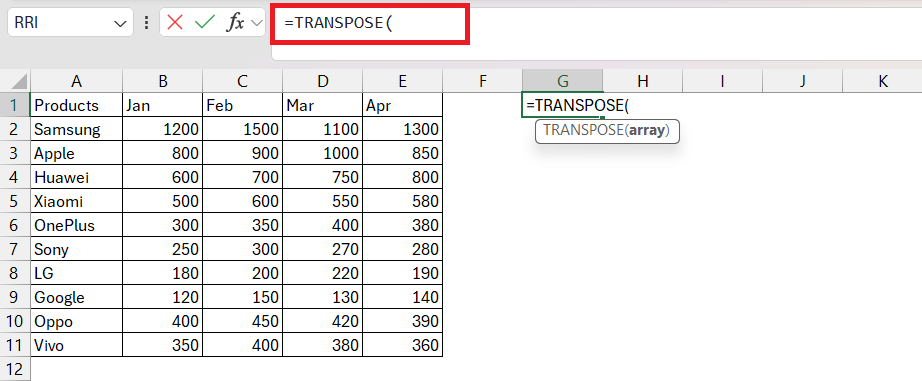
STEP 2: Enter the TRANSPOSE function.

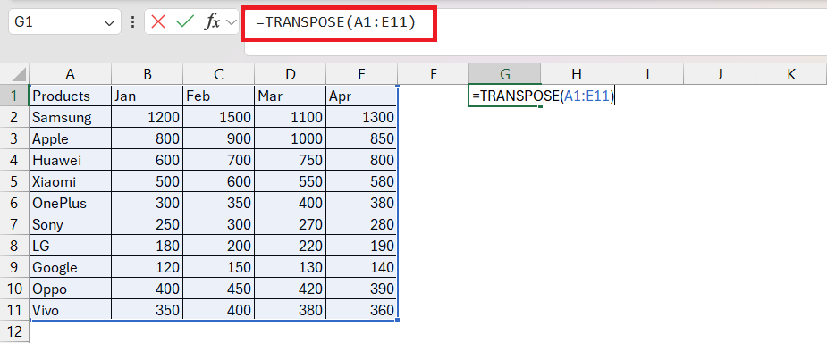
STEP 3: Enter the argument i.e. range. Here, it is A1:E11.

Your data has been transposed correctly.

This method is useful when you want the transposed data to update dynamically with changes in the original dataset. Suppose, you change the value for Xiaomi sales for January to 1500 in the original data (i.e. B5), the transposed data will also be changed (i.e. K2).

 

Method 3 – Power Query

Power Query is a powerful and flexible way to handle large datasets and can be used to transpose data easily. Here’s a step-by-step guide on how to transpose data using Power Query –

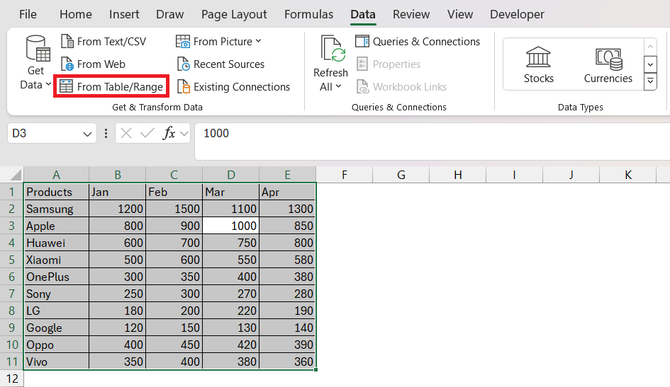
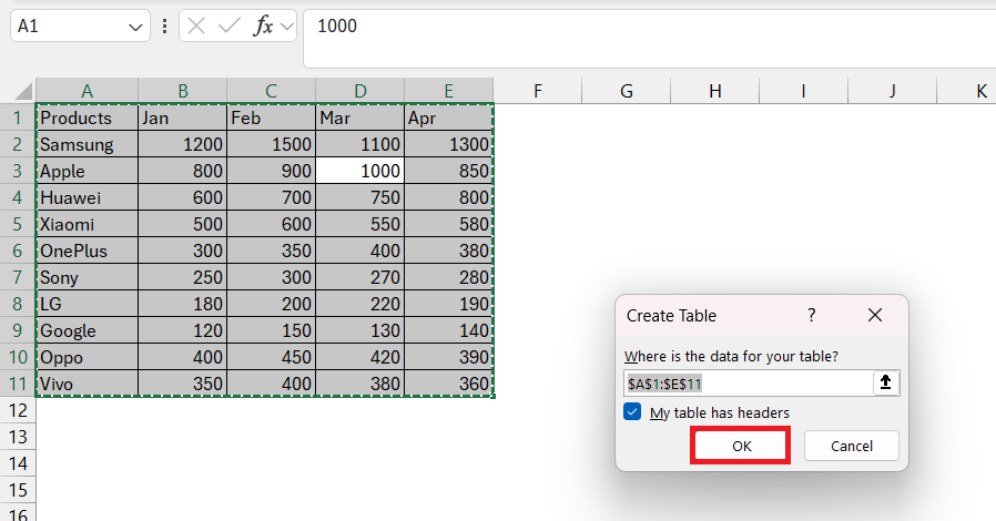
STEP 1: Select the sales data and go to Data > From Table/Range.

STEP 2: In the dialog box, select OK.

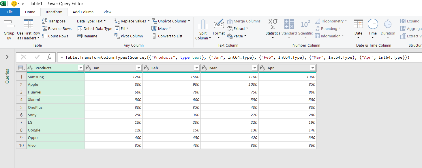
In the Power Query Editor, you’ll see a table representing your data.

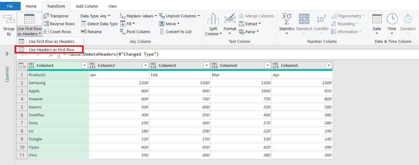
STEP 3: Go to Transform > Use Headers as First Row.

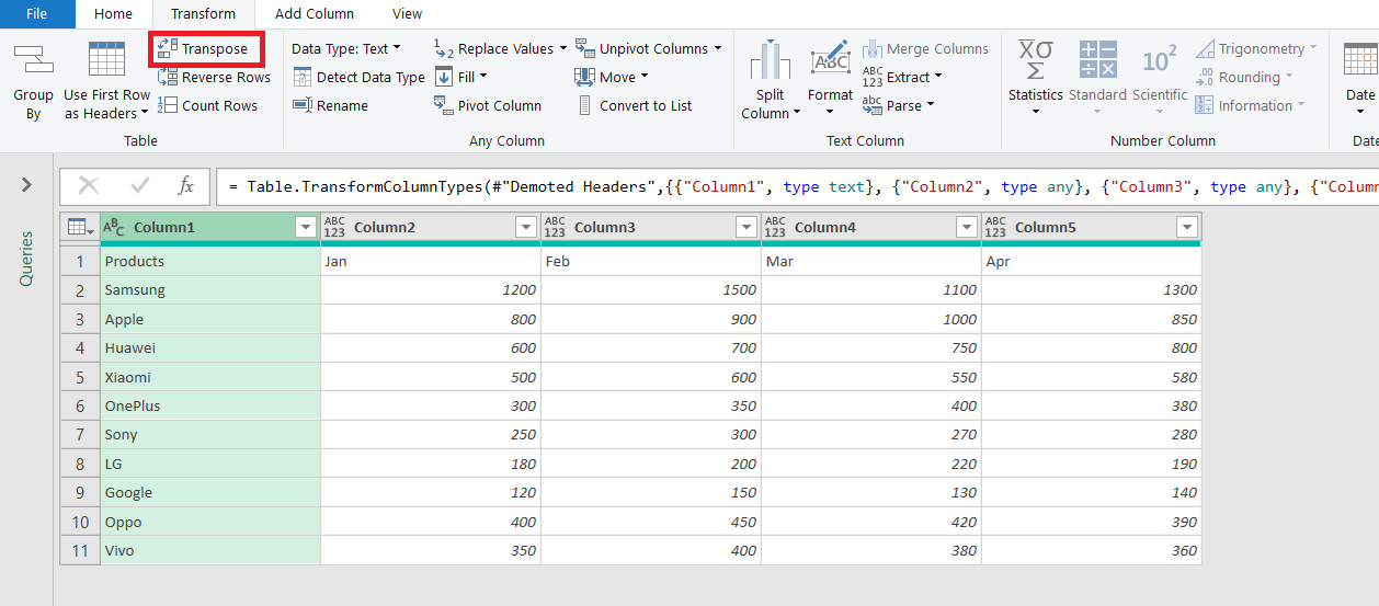
STEP 4: Go to Transform > Transpose.

The rows will be converted to columns and columns will be converted to rows.

STEP 5: Go to Transform > Use First Row as Headers.

The first row will now become the header.

STEP 6: Go to Home > Close & Load.

The transposed data will be displayed in the new worksheet.

 

In conclusion, Excel’s TRANSPOSE feature is a valuable tool for data analysts and professionals working on data manipulation.

This article has provided a comprehensive overview of three methods for transposing data in Excel – quick and straightforward Paste Special option, the dynamic TRANSPOSE function, and the powerful and flexible Power Query.

Learn more about Power Query with our 50 Things You Can Do With Excel Power Query.