Now, let’s explore each of these steps individually!
Download the Excel Workbook below to follow along and start Unleashing the Power of Pivot Tables in Excel –
download excel workbookPivot-Table.xlsx
Pivot Tables Superpower: Answering Questions
Consider the example below. Let’s say we wanted to answer the question What is the amount sold by each salesperson? Answering it could be time consuming and difficult because each salesperson appears on multiple rows, and we would need to total all of their different orders individually. This is where a pivot table will come in handy.
With Pivot Tables, we can easily calculate and summarize our data. Our final Pivot Table will look like this:
Creating a Pivot Table
Now, let’s create the pivot table.
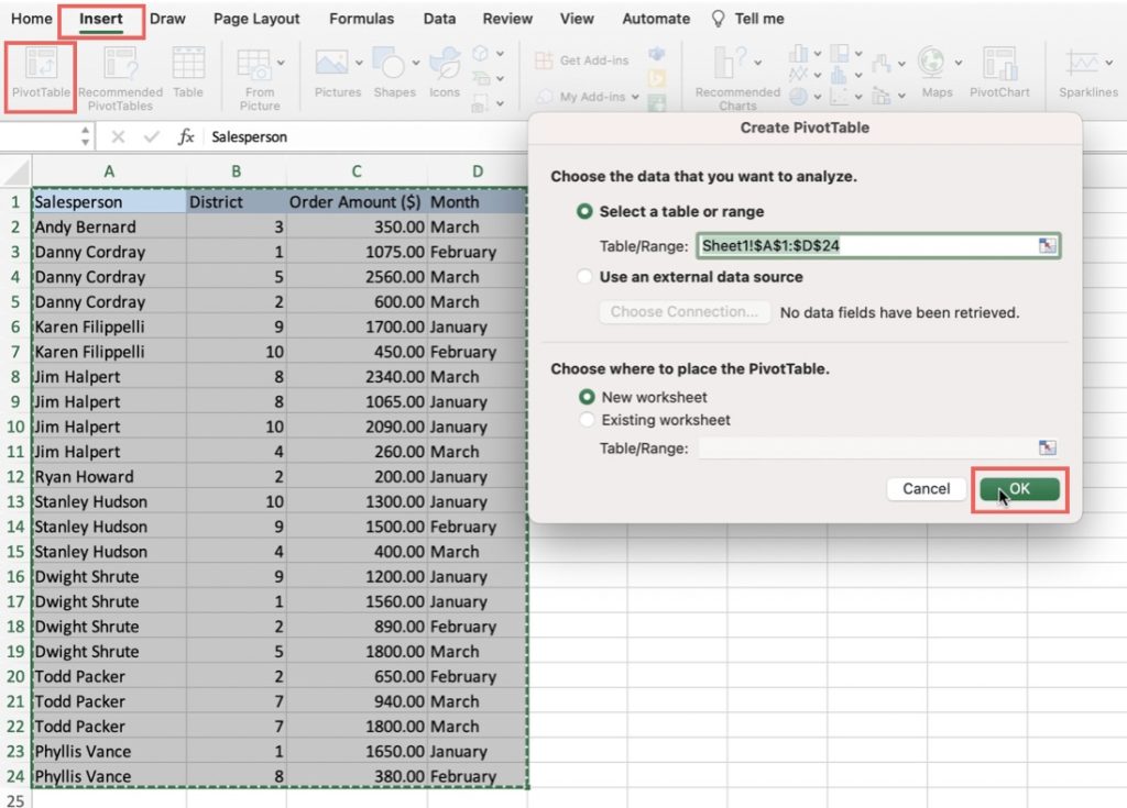
Select the dataset, including all four fields.
Go to the Insert tab and click on PivotTable.
In the PivotTable dialog box, ensure that the correct range is selected and choose where you want to place the pivot table. For this example, choose a New Worksheet.
Click OK to create the pivot table.
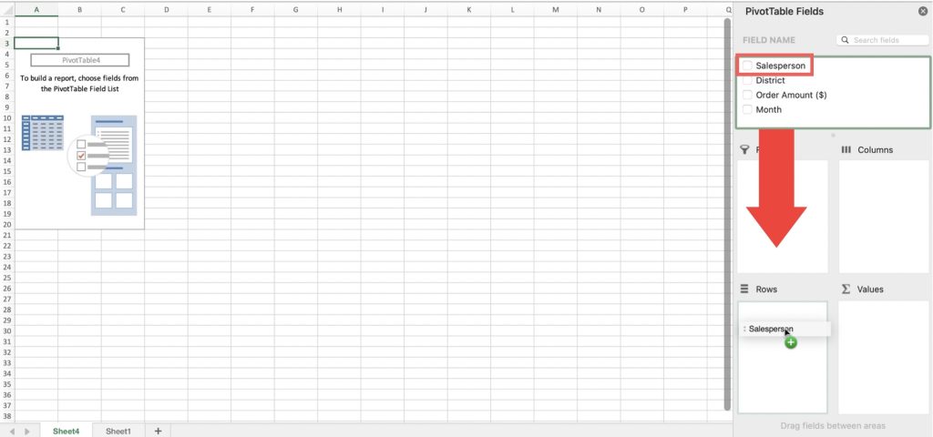
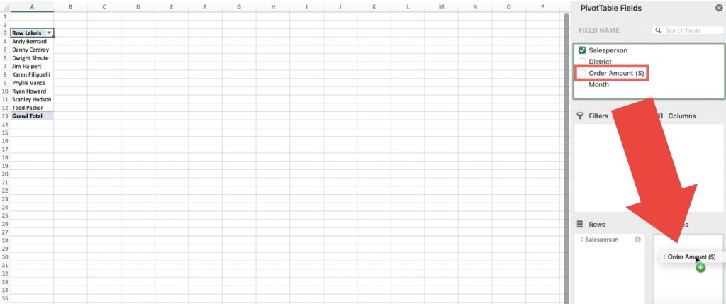
In the PivotTable Field List pane on the right, drag and drop the fields into the desired areas:
Drag the Salesperson field to the Rows area.
Drag the Order Amount field to the Values area.
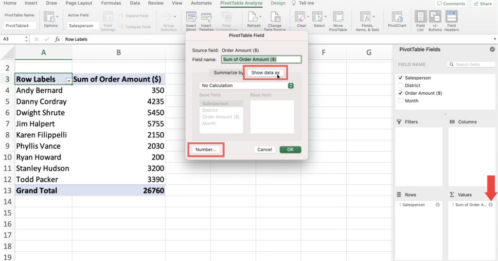
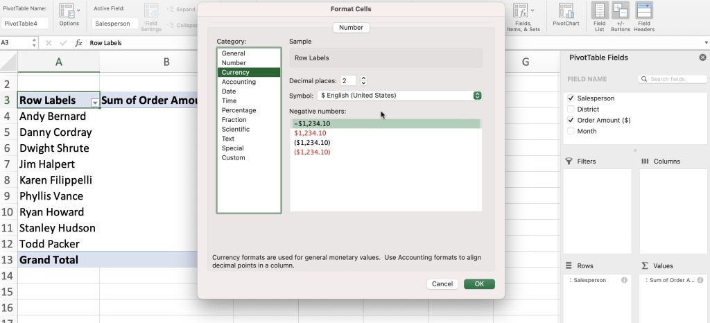
If you want to change the summary calculation, you can click on the dropdown arrow next to Sum of Order Amount in the Values area, select Value Field Settings, and choose a different calculation, such as average or count. Furthermore, you can change the number format to reflect the currency of your data.
Your pivot table is now set up. It will display the Sum of Order Amount by each Salesperson, along with its’ grand total.
Reminder: If you need to change the data in your source worksheet, the PivotTable won’t update automatically. To ensure the PivotTable reflects the latest data, you need to manually update it by selecting the PivotTable and then go to the Analyze tab, then click the Refresh button.
Adding Columns to the Pivot Table
To add columns to a pivot table, follow these steps:
Select the pivot table in Excel.
In the PivotTable Field List pane on the right, locate the Columns area.
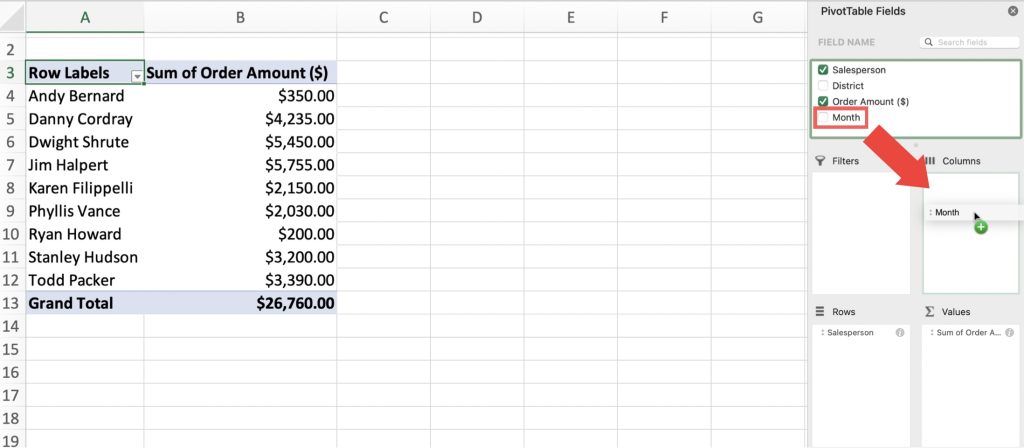
Drag the desired field, such as Month, from the PivotTable Field List and drop it into the Columns area.
The pivot table will automatically update, adding a column for the selected field. In this case, the column would represent different the different months.
Excel will adjust the pivot table layout to include the new columns, providing a comprehensive view of the data across the added dimensions.
Changing a Row or Column
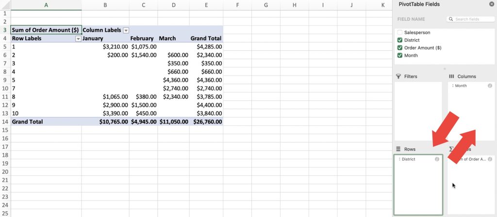
To change a row field, click and drag the desired field from the Rows area in the PivotTable Field List pane to the Columns area. For example, you can drag the Month field from the Rows area to the Columns area.
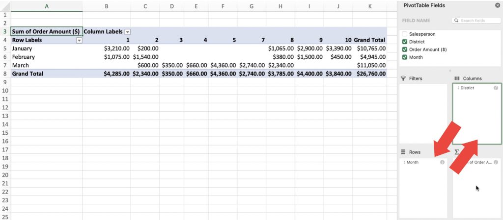
To change a column field, click and drag the desired field from the Columns area in the PivotTable Field List pane to the Rows area. For example, you can drag the Month field from the Columns area to the Rows area.
As you drag and drop the fields, the pivot table will automatically update to reflect the changes, reorganizing the data accordingly. The row and column fields will be swapped, resulting in a different layout for the pivot table.
There you have it! The pivot table feature in Excel empowers users to efficiently summarize and analyze extensive datasets. By quickly organizing, grouping, and calculating data, it lets users gain new perspective on the data.
John Michaloudis is a former accountant and finance analyst at General Electric, a Microsoft MVP since 2020, an Amazon #1 bestselling author of 4 Microsoft Excel books and teacher of Microsoft Excel & Office over at his flagship MyExcelOnline Academy Online Course.


