In Power Pivot, one of the major and more powerful feature are Measures.
Measures (also known as Calculated Fields in Excel 2013) are formulas/calculations that are added to a Pivot Table.
We will work on a simple example to show you how easy it is to use the COUNTROWS function in your Measure.
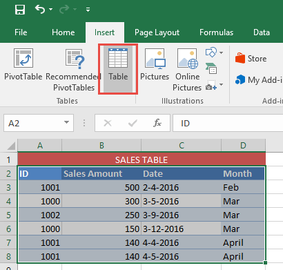
STEP 1: Select the Sales Table. Go to Insert > Table. Click OK.
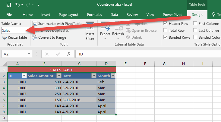
STEP 2: Go to Table Tools > Design > Table Name and give your new Table a descriptive name. In our example, we will name it Sales
STEP 3:
In Excel 2013 & 2016
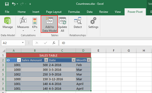
Select your Sales Table. Go to Power Pivot > Add to Data Model.
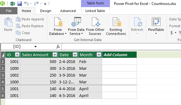
This will import your new Table into the Power Pivot Window.
In Excel 2010
Go to PowerPivot > Create Linked Table.
STEP 4: This will open the Power Pivot Window.
The Sales Table will now be automatically loaded to the Power Pivot Data Model.
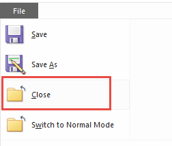
Now Close the Power Pivot Window.
STEP 5: Go to Insert> Pivot Table.
In Excel 2016
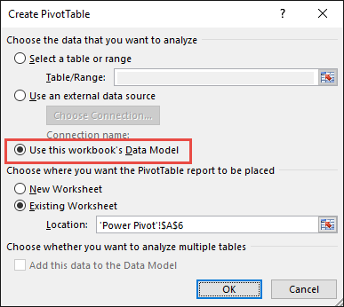
Select Use this workbook’s Data Model. This will use the Data Model you just uploaded in the last step.
Select Existing Worksheet and choose your location for your Pivot Table and press OK.
In Excel 2013
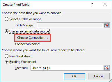
Go to Use External Data Source > Choose a Connection
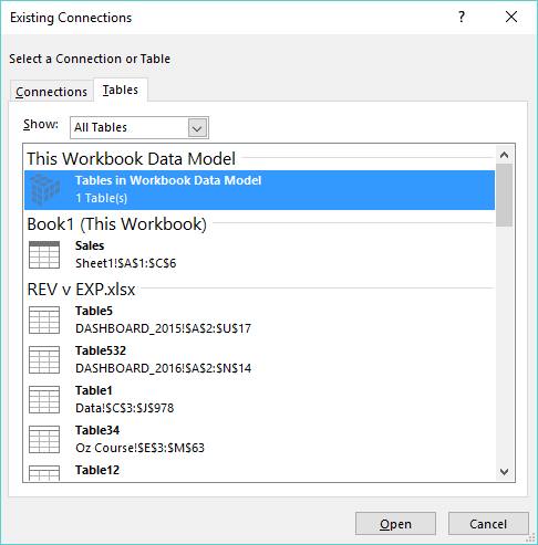
Now select Tables > This Workbooks Data Model > Open:
In Excel 2010
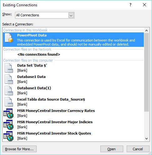
Go to Use an External Data Source > Choose Connection:
Now select PowerPivot Data > Open:
STEP 6: Adding a Measure:
In Excel 2016
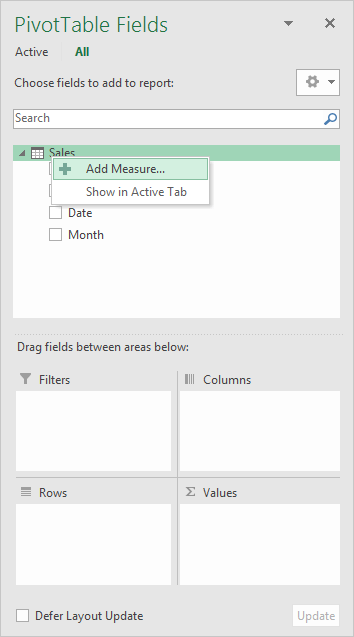
On the Sales Table, right click and select Add Measure.
An alternative way in Excel 2016 is go to Power Pivot > Measures > New Measure.
In Excel 2013
Go to PowerPivot > Calculated Fields > New Calculated Field
(In Excel 2013 “Measures” were renamed “Calculated Fields” and returned to “Measures” in Excel 2016…I know, how annoying!)
In Excel 2010
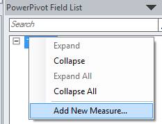
On the Sales table, right click and select Add New Measure.
An alternative way in Excel 2010 is to select a cell inside the Pivot Table that was created in the previous step and go to Power Pivot > New Measure:
STEP 7: This is where we create our Measure using the COUNTROWS function.
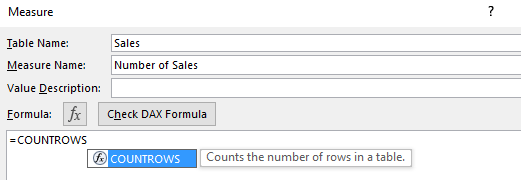
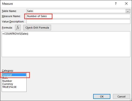
For Measure Name, type in any name that you like e.g. Number of Sales
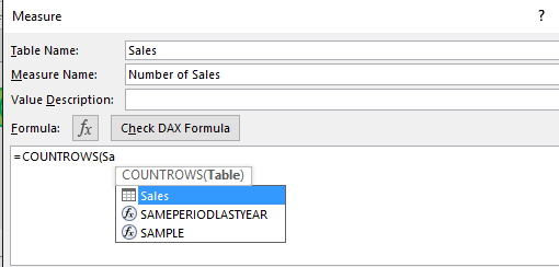
For the Formula, after the = sign start typing the word COUNTROWS.
Just like in native Excel, this will bring up the Formula helper and choose the COUNTROWS function by either double clicking on the blue highlighted COUNTROWS option or by pressing the Tab keyboard to confirm this suggestion:
After the COUNTROWS formula is selected, type in the Table name that we created in Step 2, which we called Sales.
This will bring up the Formula helper and within here you need to select the Sales Table option and close the parenthesis:
Set the Category as General, and this will automatically handle the formatting for you. Press OK to confirm this.
This Measure will now return the Total Number of Rows based on the Pivot Table we will be setting up in the next step.
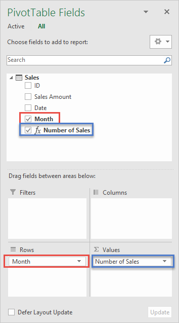
STEP 8: Place your new Measure Number of Sales in the Values area.
Then place Month in the Rows area
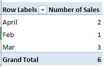
STEP 9: Now we are able to use our new COUNTROW Measure in the Pivot Table.

Bryan
Bryan Hong is an IT Software Developer for more than 10 years and has the following certifications: Microsoft Certified Professional Developer (MCPD): Web Developer, Microsoft Certified Technology Specialist (MCTS): Windows Applications, Microsoft Certified Systems Engineer (MCSE) and Microsoft Certified Systems Administrator (MCSA).
He is also an Amazon #1 bestselling author of 4 Microsoft Excel books and a teacher of Microsoft Excel & Office at the MyExecelOnline Academy Online Course.

