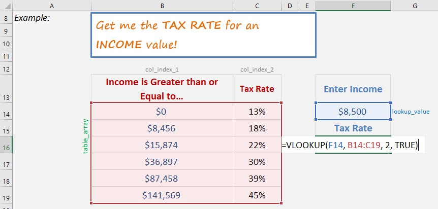
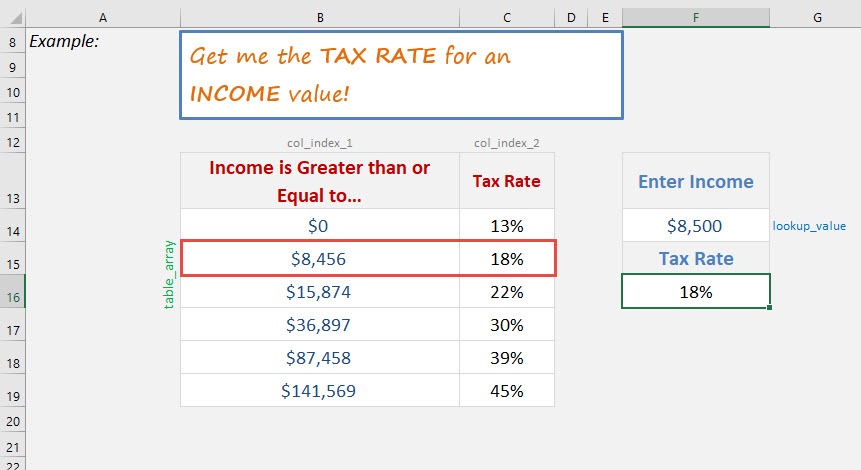
The Vlookup function in Excel is great when you want to find an exact match in your data table but what happens if you want to find an approximate match? Approximate matches are used when you have an ascending table like Commission Bonus Rates or Income Tax Rates. IMPORTANT: For the Vlookup Approximate Match to work in Excel, the table_array has to be sorted in ascending order! So the way that this formula works is that it looks at the first value in the Table_Array that is greater than the Lookup_Value and then goes back one value.
Key Takeaways
-
VLOOKUP Approximate Match Finds Closest Value – When set to TRUE (or omitted), VLOOKUP returns the closest value less than or equal to the lookup value.
-
Requires Sorted Data – For the approximate match to work correctly, the first column of the table must be sorted in ascending order.
-
Great for Range-Based Lookups – Ideal for grading systems, commission rates, tax brackets, or any scenario where values fall within defined ranges.
-
Faster Than Exact Match – Approximate match searches are quicker and more efficient on large datasets compared to exact matches.
-
Defaults to Approximate Match – If the 4th argument is left blank, VLOOKUP defaults to approximate match, which can cause errors if the data isn’t sorted.
Table of Contents
Quick Overview
What does it do?
Searches for an approximate value in the first column of a table array and returns a value in the same row from another column (to the right) in the table array.
Formula breakdown:
=VLOOKUP(lookup_value, table_array, col_index_num, [range_lookup])
What it means:
=VLOOKUP(this value, in this list, and get me value in this column, Approximate Match/TRUE/1])
Want to know how to use the VLOOKUP function from Beginner to Advanced?
*** Watch our video and step by step guide below with free downloadable Excel workbook to practice ***
Watch it on YouTube and give it a thumbs-up!
Want to know how to use VLOOKUP with Approximate Match?
*** Watch our video and step by step guide below with free downloadable Excel workbook to practice ***
Have a look at the following tutorial which explains this formula & don’t forget to download the workbook so you can practice:
How to Use Vlookup Approximate Match in Excel
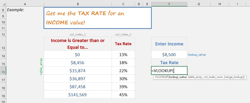
=VLOOKUP(
STEP 2: The VLOOKUP arguments:
Lookup_value
What is the value to be looked up?
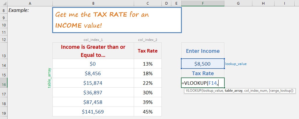
Select the cell that contains the income as the lookup value.
=VLOOKUP(F14,
Table_array
Where is the list of data?
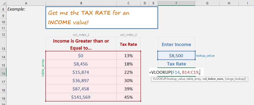
Select the tax table, as that is where our formula is going to get the tax rate.
=VLOOKUP(F14, B14:C19,
Col_index_num
Which column in the table_array contains the data you want to return?
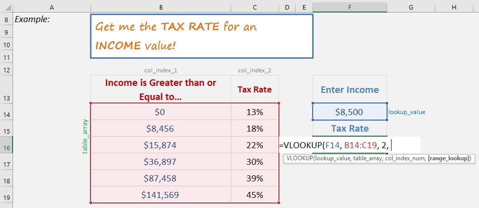
We want the tax rate which is the second column.
=VLOOKUP(F14, B14:C19, 2,
[Range_lookup]
Would it be an approximate match?
Set this to TRUE as we want an approximate match.
=VLOOKUP(F14, B14:C19, 2, TRUE)
You now have your tax rate!
Frequently Asked Questions
What is VLOOKUP approximate match used for?
It’s used when you want to find the closest value without exceeding the lookup value, perfect for scenarios like tax rates, grading, or tiered pricing.
How do I enable approximate match in VLOOKUP?
Set the 4th argument to TRUE or leave it blank. Example:=VLOOKUP(A2, B2:D10, 2, TRUE)
Does the data need to be sorted for approximate match?
Yes, the first column of your lookup range must be sorted in ascending order; otherwise, VLOOKUP may return incorrect results.
What happens if I use approximate match on unsorted data?
The result may be incorrect or unpredictable because VLOOKUP assumes sorted data when performing an approximate match.
Can I use approximate match with text values?
No, approximate match is designed for numeric ranges. For text lookups, it’s best to use exact match (FALSE).
John Michaloudis is a former accountant and finance analyst at General Electric, a Microsoft MVP since 2020, an Amazon #1 bestselling author of 4 Microsoft Excel books and teacher of Microsoft Excel & Office over at his flagship MyExcelOnline Academy Online Course.


