How to Use VLOOKUP between Sheets

In many cases, your data may be connected but spread out among different sheets. With the help of VLOOKUP between sheets, you can overcome this obstacle and extract corresponding data from different sheets. This gives you the freedom to have data in multiple sheets and not face restrictions in using them.

Key Takeaways:

• Cross-Sheet Data Lookup: The VLOOKUP function can retrieve data from a different sheet by referencing the sheet name in the formula. This is useful for linking and analyzing data stored across multiple worksheets.
• Syntax for Cross-Sheet Lookup: The formula format for using VLOOKUP between sheets is:
  =VLOOKUP(lookup_value, SheetName!table_array, col_index_num, [range_lookup]), where SheetName!table_array specifies the range in the source sheet.
• Sheet Name with Spaces: If the sheet name contains spaces or special characters, enclose it in single quotes when referencing it in the formula (e.g., 'Sheet 2'!A1:C10).
• Dynamic Range Updates: Using named ranges or dynamic ranges in the source sheet ensures that the VLOOKUP formula automatically adjusts when the table array expands or changes.
• Absolute References for Stability: Use absolute references (e.g., $A$1:$C$10) for the table_array argument to prevent errors when copying the formula across cells. This ensures consistent data retrieval from the intended range.

VLOOKUP Syntax

What does it do?

Searches for a value in the first column of a table array and returns a value in the same row from another sheet´s column (to the right) in the table array.

Formula breakdown:

=VLOOKUP(lookup_value, table_array, col_index_num, [range_lookup])

What it means:

=VLOOKUP(this value in Sheet1, in this list in Sheet2, and get me value in this column in Sheet2, Exact Match/FALSE/0])

Sometimes you are faced with a situation where you have a list of data and you want to bring in complementary data from a different sheet within the same workbook.

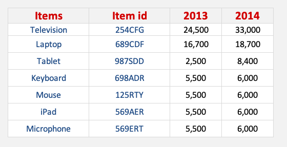
Let’s say that you have a list of “items” in a table within Sheet1 and you want to bring in their corresponding “item id’s” from Sheet2.

You can manually copy and paste the item id’s from Sheet2 to Sheet1 but that would take too long and you are also prone to errors.

The quick and error-proof way is by using the VLOOKUP function.

So, let’s dive in and learn how to use VLOOKUP between sheets!

 

VLOOKUP from another sheet

Follow the step-by-step tutorial on how to VLOOKUP for multiple sheets with example and download this Excel workbook to practice along:

Download workbookVlookup_Different-Sheetv2s.xlsx

 

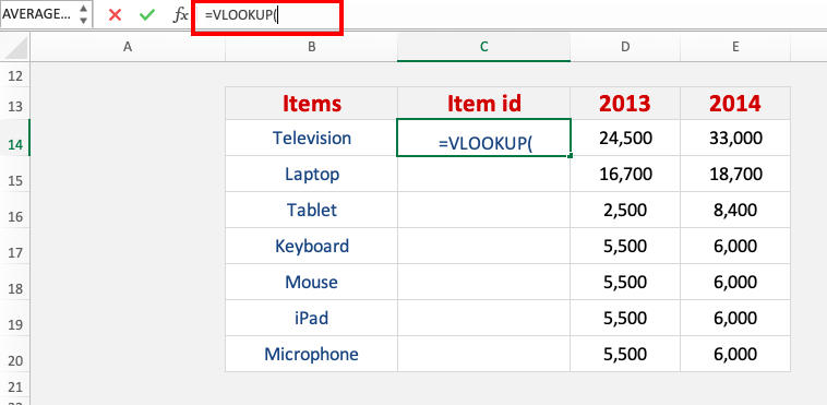
STEP 1: We enter the VLOOKUP function in the blank cell where we need to extract the data

=VLOOKUP(

 

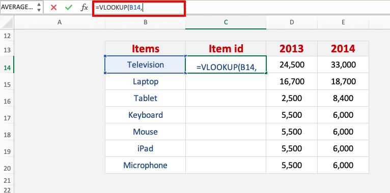
STEP 2: Enter the first argument for VLOOKUP – Lookup_value

What is the value that you want to look for?

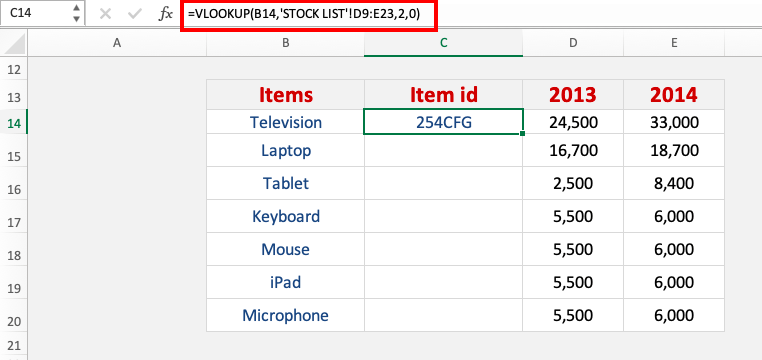
In our example, it is Television, so select that in the “Items” column

=VLOOKUP(B14,

 

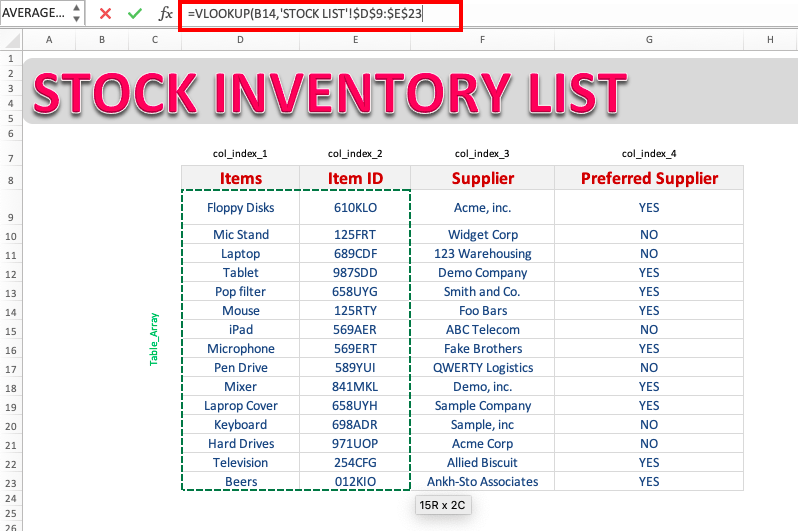
STEP 3: Enter the second argument for VLOOKUP – Table_array

What is the table or range that contains your data?

Select the Stock inventory table in the stock list sheet so that the VLOOKUP formula will search there

=VLOOKUP(B14,‘STOCK LIST’!D9:E23,

Ensure that you press F4 so that you can lock the table range.

=VLOOKUP(B14,‘STOCK LIST’!$D$9:$E$23,

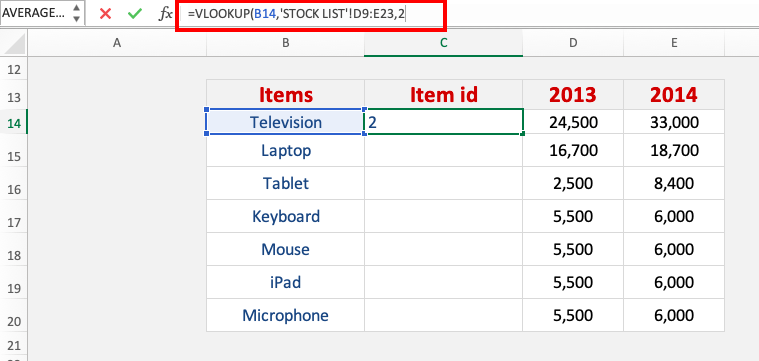
STEP 4: Enter the third argument for VLOOKUP – Col_index_num

What is the column that you want to retrieve the value from?

Since we want to retrieve the item id we will write 2, as the item id is the second column in the table array that we selected

=VLOOKUP(B14,’STOCK LIST’!D9:G23,2

 

STEP 4: Enter the fourth argument for VLOOKUP – Range_lookup

What kind of matching do you need?

We want an exact match of the Television text so make sure FALSE OR 0 is selected.

=VLOOKUP(B14,’STOCK LIST’!D9:G23,2,0)

Apply the same formula to the rest of the cells by dragging the lower right corner downwards.

You now have all of the results!

In this example, you have learned how to pull data from another worksheet in the same workbook using VLOOKUP from multiple sheets. Excel also allows you to get data from another workbook from your computer.

Let’s see how that is done!

 

VLOOKUP from another workbook

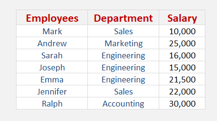
Suppose you have monthly sales data in one workbook and you have the employee name and data in another workbook.

You have to link these two workbooks using VLOOKUP to extract values for a better and cohesive database.

 

In this tutorial, we will show you how you can use VLOOKUP across different Excel workbooks and link and extract data easily.

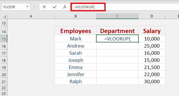
Step 1: We enter the VLOOKUP function in the blank cell where we need to extract the data

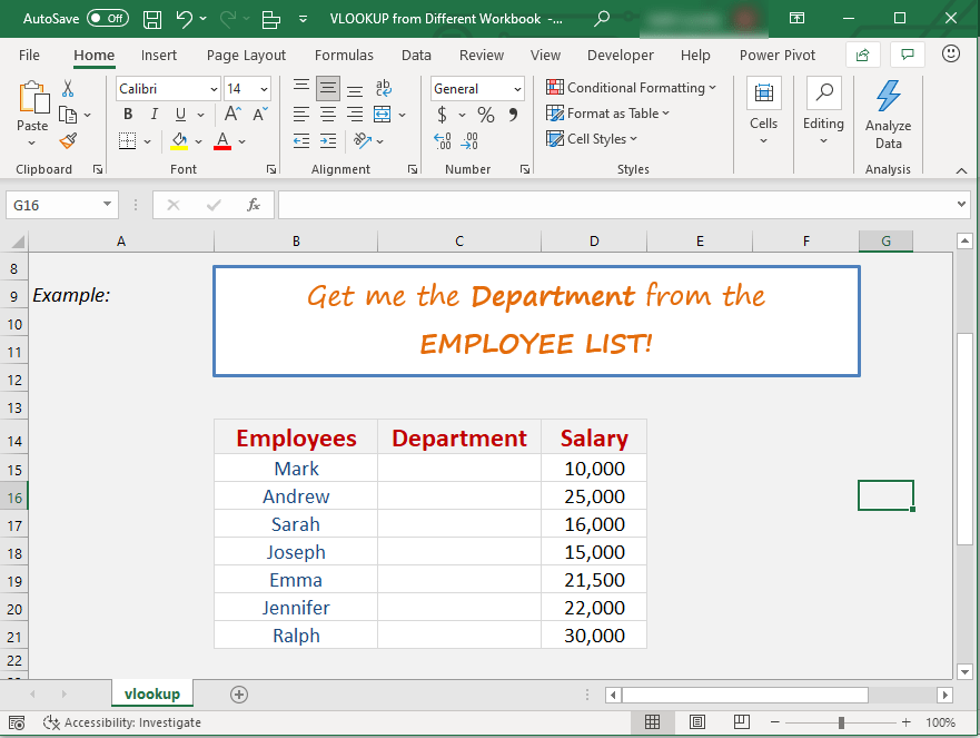
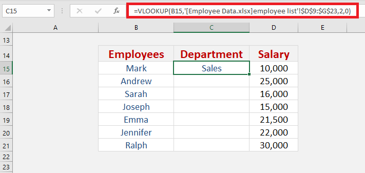
This is the cell where we want the corresponding data. In our case, this is the department of the employee in cell C15.

=VLOOKUP(

 

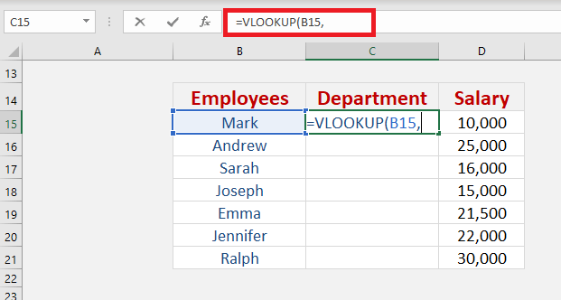
Step 2: Enter the first argument of the VLOOKUP function – Lookup_value

What is the value that you want to look for?

It is the value to be found in the first column of the table. It can be a value, text string, or reference.

In our example, it is Mark, so select that in the “Employees” column

=VLOOKUP(B15,

 

Step 3: Enter the second argument of the VLOOKUP function – Table_array

What is the table or range that contains your data?

It is a table of logical values, texts, numbers from which the data is retrieved

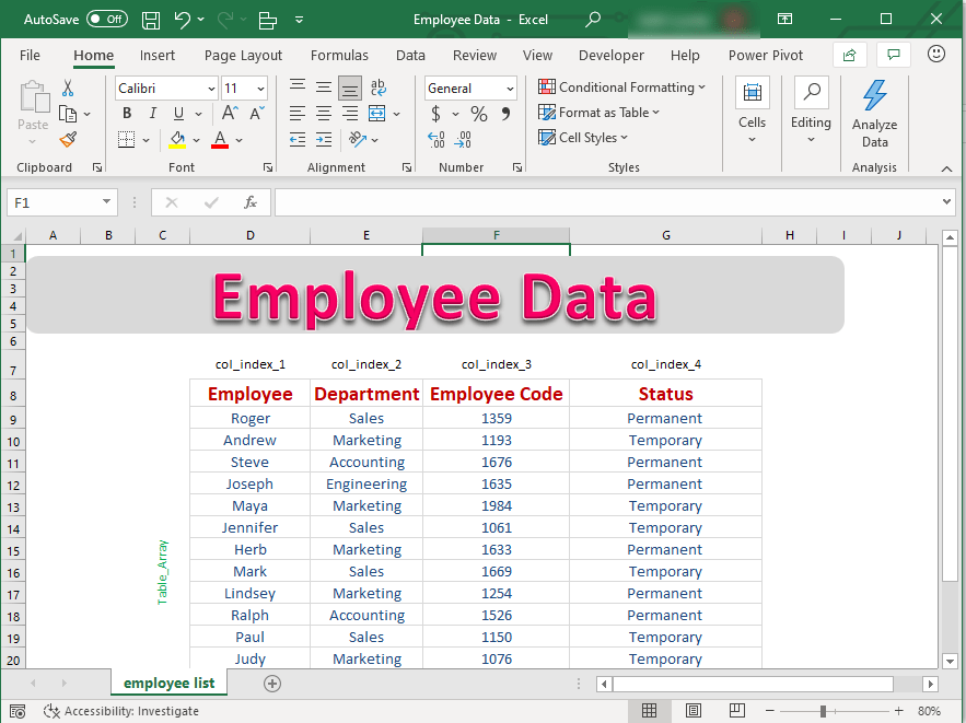
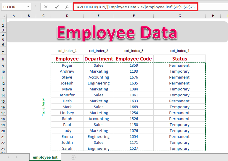
Here you need to go to the workbook where your employees’ data is stored so that we can get the name of the department they are associated with.

Select the data table containing the names and departments of the employees.

Ensure that you press F4 so that you can lock the table range. You will be sure the range is locked when $ signs appear.

=VLOOKUP(B15,‘[Employee Data.xlsx]employee list’!$D$9:$G$23

 

Notice how the name of the different workbooks appears between square brackets. This is the indication that the reference is from another workbook.

So if you are typing out the formula make sure to include the square brackets.

 

Step 4: Enter the third argument of the VLOOKUP function – Col_index_num

What is the column that you want to retrieve the value from?

It is the column number from which the matching value should be returned.

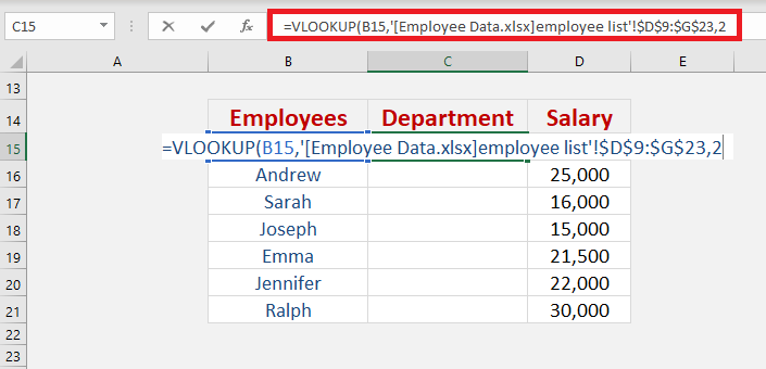
Since we want to retrieve the Department name we will write 2, as the department name is the second column in the table array that we selected.

Similarly, if we wanted to extract the employee code, we would type 3 here as employee code is in the third column of the table that we selected.

=VLOOKUP(B15,'[Employee Data.xlsx]employee list’!$D$9:$G$23,2

 

 

Step 5: Enter the fourth argument of the VLOOKUP function – Range_lookup

What kind of matching do you need?

To find a perfect match, we need to select FALSE here.

In case the data is arranged in ascending order and belongs to a certain range/period, then TRUE should be selected to get the closest match.

We want an exact match of Mark text so make sure FALSE or 0 is selected.

=VLOOKUP(B15,'[Employee Data.xlsx]employee list’!$D$9:$G$23,2,0)

 

Apply the same formula to the rest of the cells by dragging the lower right corner downwards.

This is how you can extract values using VLOOKUP in multiple sheets or multiple workbooks!

Frequently Asked Questions

How can I use VLOOKUP to retrieve data from another sheet in Excel?
To use VLOOKUP across sheets, include the sheet name in the table array. For example:
=VLOOKUP(A2, Sheet2!A1:C10, 2, FALSE)
In this formula, Sheet2!A1:C10 specifies the range in the second sheet, from which VLOOKUP retrieves the data.

What should I do if the sheet name has spaces or special characters?
If the sheet name contains spaces or special characters, enclose the sheet name in single quotes in your formula. For example:
=VLOOKUP(A2, 'Sales Data'!A1:D10, 3, TRUE)

Why is my VLOOKUP returning a #N/A error when referencing another sheet?
The #N/A error usually occurs if the lookup_value doesn’t exist in the first column of the table array, or if the table array range is incorrect. Ensure the lookup value matches exactly (case-insensitive) and check that the referenced range includes the required data.

Can I use VLOOKUP between sheets in different Excel workbooks?
Yes, you can use VLOOKUP between workbooks. Reference the external workbook in your formula using its file name, like this:
=VLOOKUP(A2, '[Workbook2.xlsx]Sheet1'!A1:C10, 2, FALSE)
Make sure the referenced workbook is open; otherwise, you’ll see a #REF! error.

How do I ensure the table array remains stable when copying the VLOOKUP formula?
Use absolute references for the table array by adding dollar signs (e.g., $A$1:$C$10). This ensures that the table range does not change when you drag the formula to other cells. For example:
=VLOOKUP(A2, Sheet2!$A$1:$C$10, 2, FALSE)