Mastering VLOOKUP with Multiple Criteria in Excel – 3 Quick and Easy Methods

VLOOKUP is used to search for a value in the first column of a table array and return a value in the same row from another column. But what happens when we want to search for a value based on multiple criteria? VLOOKUP with multiple criteria has got that covered!

Before we proceed further, let us quickly go through the syntax of VLOOKUP –

Formula breakdown:
=VLOOKUP(lookup_value, table_array, col_index_num, [range_lookup])

What it means:
=VLOOKUP(this value, in this list, and get me value in this column, Exact Match/FALSE/0])

The syntax of VLOOKUP is such that it cannot natively search multiple criteria. But we can make a few tweaks to the functions and use VLOOKUP with multiple criteria to effortlessly find data and streamline the data analysis process in Excel. In this article, we will be covering 3 quick and easy methods of using VLOOKUP with multiple criteria in Excel –

Let us look at each one of these methods in detail!

Download the Excel Workbook below to follow along and understand how to use VLOOKUP with Multiple Criteria in Excel –

download excel workbookVLOOKUP-with-Multiple-Criteria.xlsx

Method 1: Helper Column

We can create a new column that concatenates the two columns containing the criteria. It is important to make sure that this column is at the beginning of the table as Excel will search the left-most column of the table array.

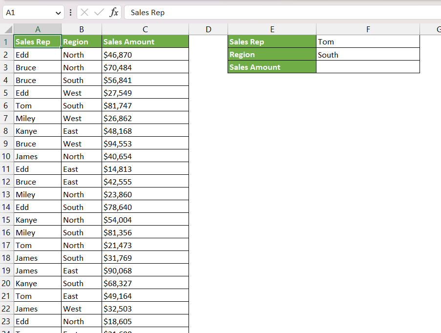
Suppose we have a dataset containing information related to sales representatives, region, and sales amount. We need to use VLOOKUP to match two criteria –

• The Sales Representative should be Tom
• The Region should be South

Follow the steps below to use VLOOKUP with multiple criteria using a helper column –

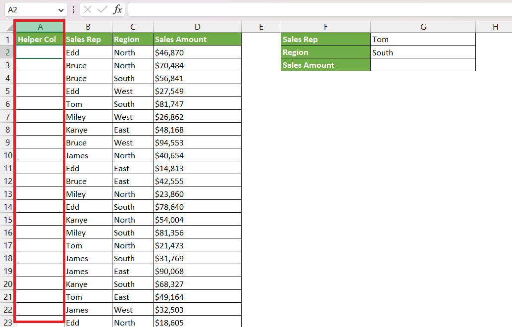
STEP 1:  Insert a Helper Column before Sales Rep Column.

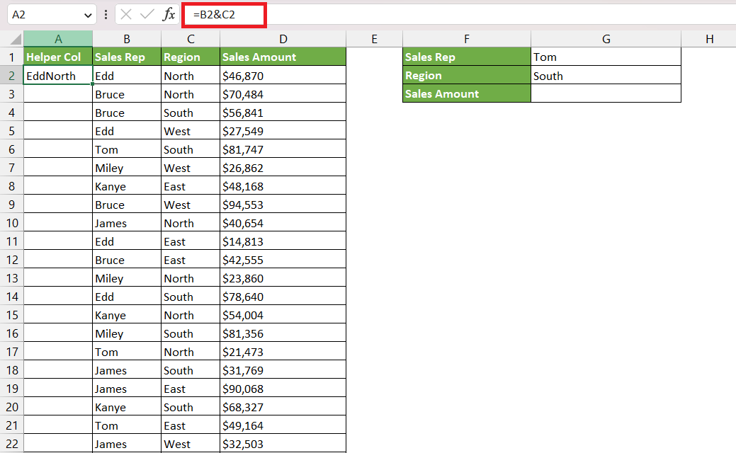
STEP 2:  Enter the following formula to concatenate the two lookup columns i.e. Sales Rep & Region

 =B2&C2

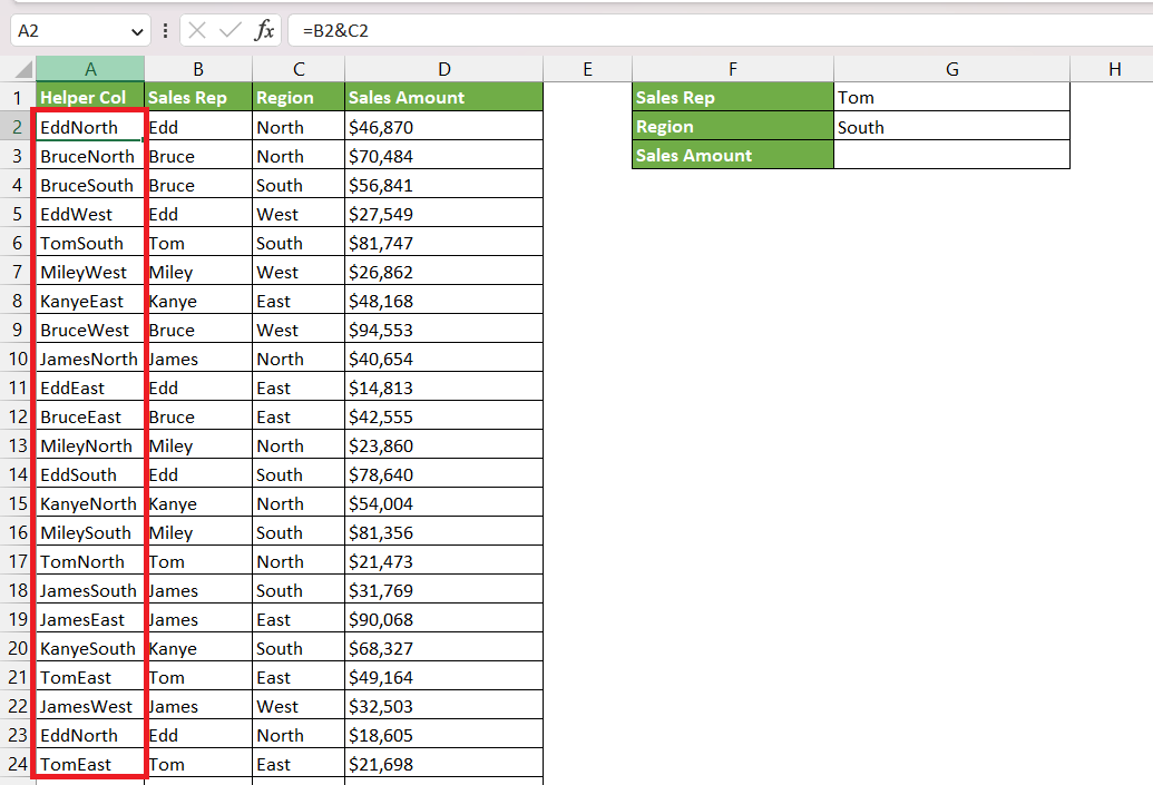
STEP 3:  Select the range A2: A25 and press Ctrl + D to copy the formula down.

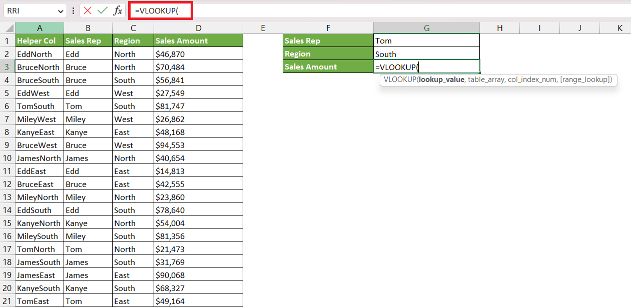
STEP 4:  Enter the VLOOKUP formula.

=VLOOKUP(

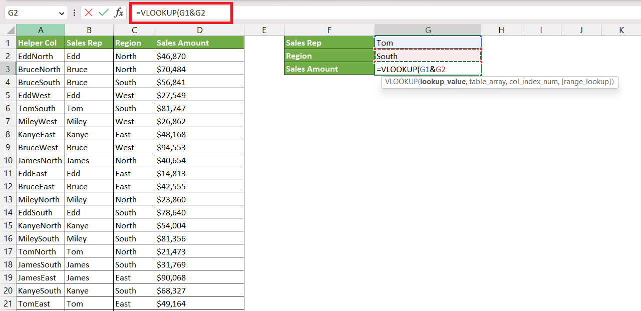
STEP 5:  Enter the first argument i.e. lookup_value. Here, it is the concatenation of cells G2 and G3 i.e. G2&G3.

=VLOOKUP(G1&G2,

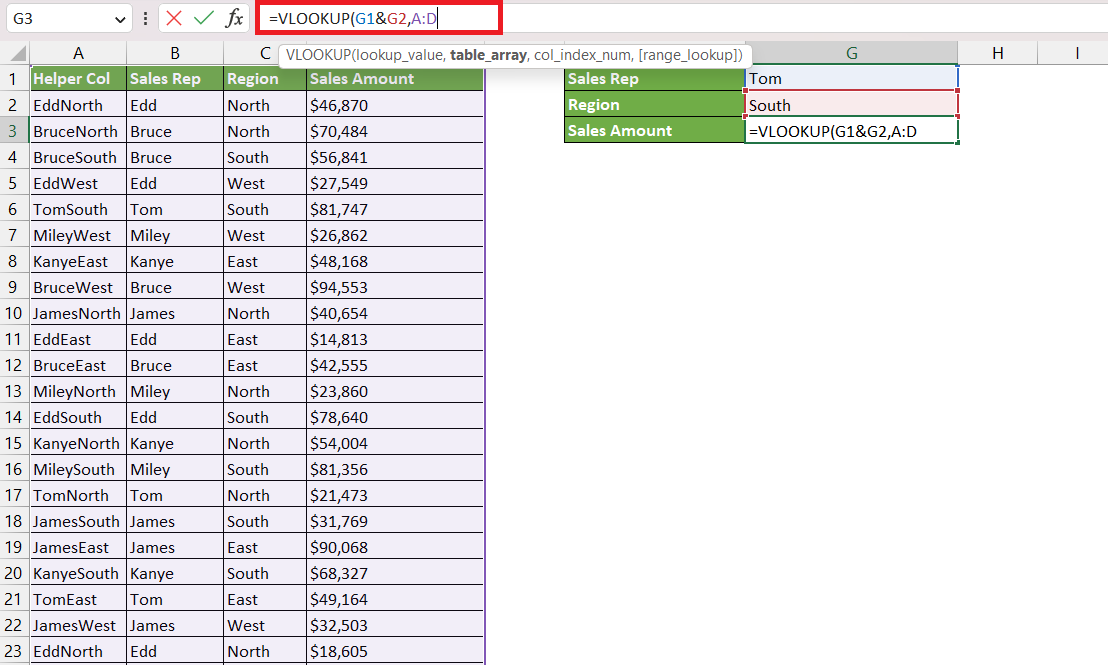
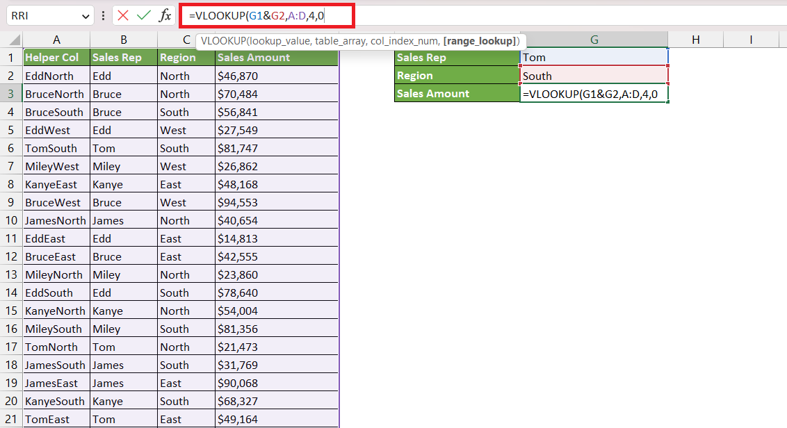
STEP 6:  Enter the second argument i.e. table_array. Here, it is the range A:D.

=VLOOKUP(G1&G2,A:D,

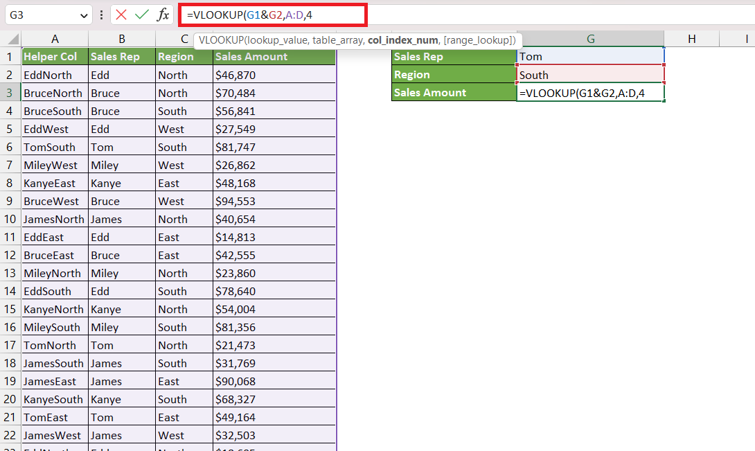
STEP 7:  Enter the third argument i.e. col_index_num. Here, it is 4 as the result is in the 4th column of the table array.

=VLOOKUP(G1&G2,A:D,4,

STEP 8:  Enter the fourth argument i.e. range_lookup. Here, it is 0 for an exact match.

=VLOOKUP(G1&G2,A:D,4,0)

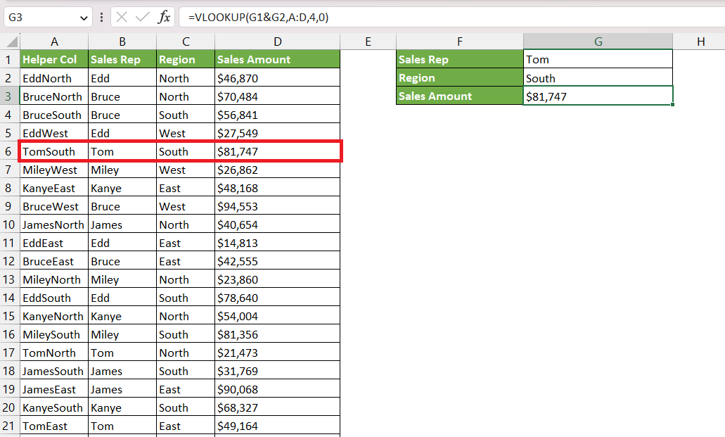
As you can see, VLOOKUP has extracted the sales amount for the sales representative named Tom in the southern region.

 

Method 2: Combination of VLOOKUP and MATCH

The MATCH function in Excel returns the position of an item within a list or a range of cells. It can be used to know in which position a certain item is located within a range.

Formula breakdown:

=MATCH(lookup_value, lookup_array, [match_type])

What it means:

=MATCH(lookup this value, from this list or range of cells, return me the Exact Match)

Let us use a combination of VLOOKUP & MATCH to get the sales amount for a sales representative named Bruce in the Eastern region –

STEP 1:  Enter the VLOOKUP function.

=VLOOKUP(

STEP 2:  Enter the first argument i.e. lookup_value. Here, it is the region that we need to find mentioned in cell H2.

=VLOOKUP(H2,

STEP 3:  Enter the second argument i.e. table_array. Here, it is A:E.

=VLOOKUP(H2,A:E,

STEP 4:  Now, we will use the MATCH function to get the column number.

=VLOOKUP(H2,A:E,MATCH(

STEP 5: Enter the first argument of the MATCH function i.e. lookup_value. Here, it is the sales representative mentioned in cell H1.

=VLOOKUP(H2,A:E,MATCH(H1,

STEP 6: Enter the second argument of the MATCH function i.e. lookup_array. Here, it is A1:E1.

=VLOOKUP(H2,A:E,MATCH(H1,A1:E1,

STEP 7: Enter the third argument of the MATCH function i.e. match_type. Here, it is 0 for an exact match.

=VLOOKUP(H2,A:E,MATCH(H1,A1:E1,0)

STEP 8: Enter the fourth argument of the VLOOKUP function i.e. range_lookup. Here, it is 0 for an exact match.

=VLOOKUP(H2,A:E,MATCH(H1,A1:E1,0),0)

The sales amount for the Bruce in the East region is extracted using the combination of VLOOKUP & MATCH –

 

Method 3: Array Function

CHOOSE function can be used to specify columns and their order for the table array used in the VLOOKUP function.

Formula breakdown:

=CHOOSE({index_num}, value1, [value2], …)

Here, we are using the array function to define the index numbers i.e. the number of columns the table should have and value1, value2, etc. is used to define the array columns. Thus, using the COLUMN function we will be able to use VLOOKUP with multiple columns.

Let us understand this using an example –

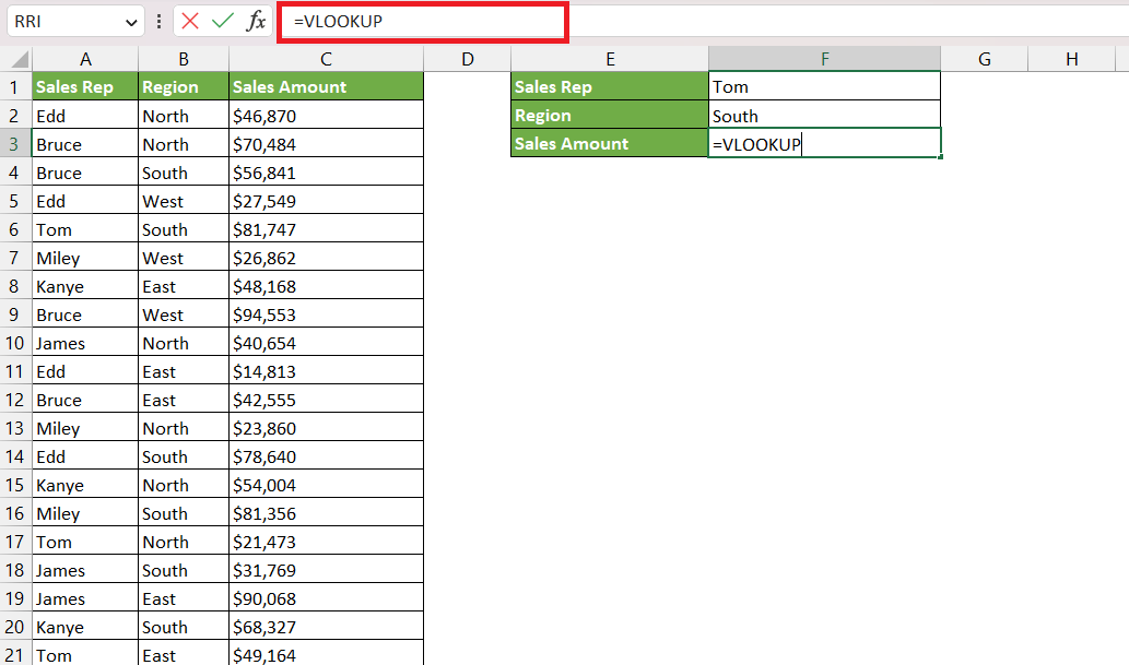
STEP 1:  Enter the VLOOKUP formula.

=VLOOKUP(

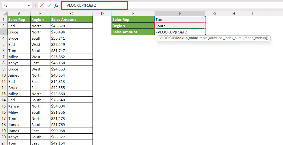
STEP 2:  Enter the first argument i.e. lookup_value. Here, it is the sales representative mentioned in cell F1 and the region mentioned in cell F2.

=VLOOKUP(F1&F2,

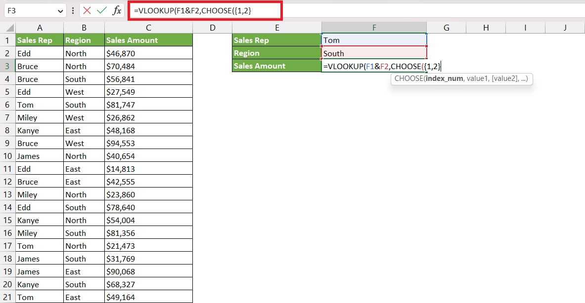
STEP 3: We will now insert CHOOSE function to get the table array. The first argument is used to define the number of columns we need to add.

=VLOOKUP(F1&F2,CHOOSE({1,2},

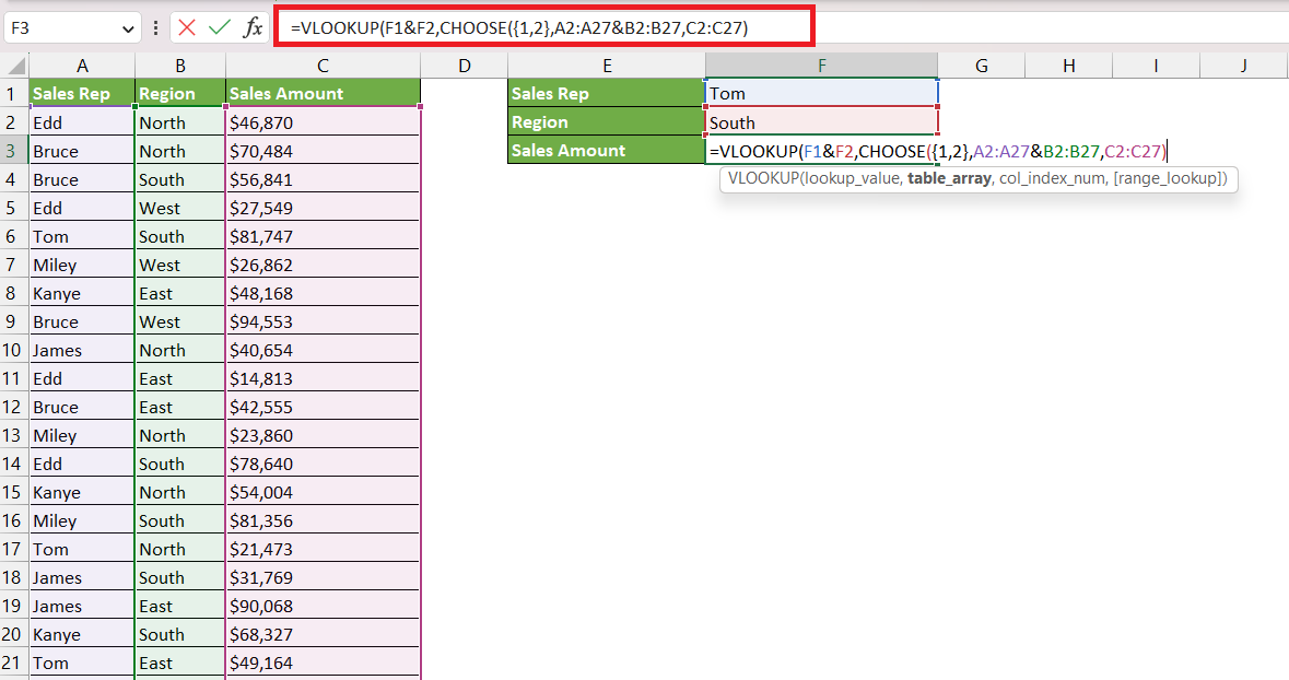
STEP 4: Enter the value arguments for CHOOSE functions i.e. the column ranges. First, we will insert the lookup columns combined using & sign and then add the result column separated by a comma.

=VLOOKUP(F1&F2,CHOOSE({1,2},A2:A27&B2:B27,C2:C27)

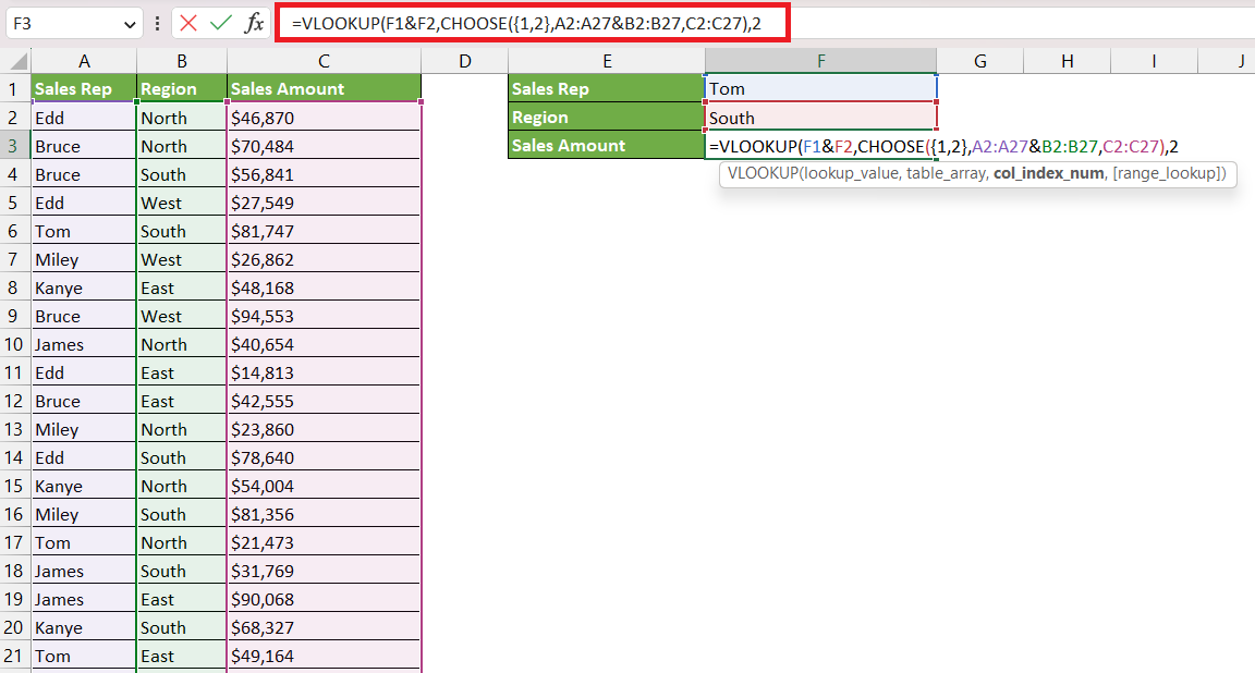
STEP 5: Enter the third argument of the VLOOKUP function i.e. col_index_num. Here, it is the 2nd column so the value will be 2.

=VLOOKUP(F1&F2,CHOOSE({1,2},A2:A27&B2:B27,C2:C27),2

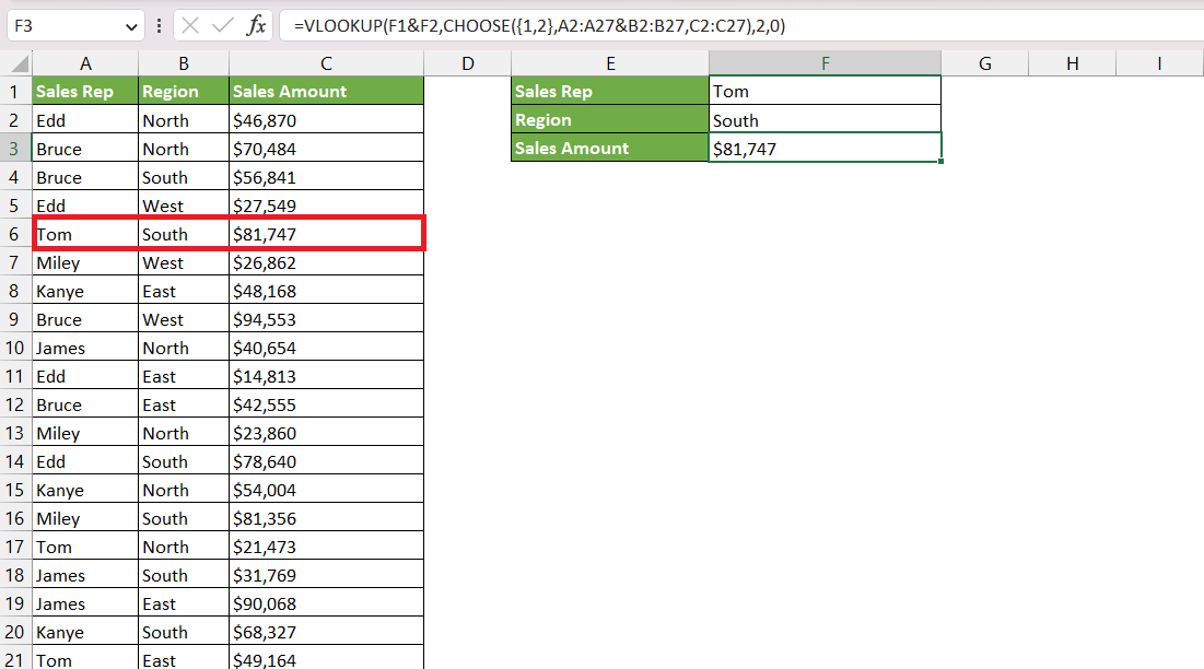
STEP 6: Enter the fourth argument of the VLOOKUP function i.e. range_lookup. Here, it is 0 for an exact match.

=VLOOKUP(F1&F2,CHOOSE({1,2},A2:A27&B2:B27,C2:C27),2,0)

As you can see, VLOOKUP has extracted the sales amount for the sales representative named Tom in the southern region.

 

Please Note – If you are working with a large dataset, it might not be a good approach to use VLOOKUP with multiple criteria. It would be better to use any of the following approaches including the INDEX MATCH function, Pivot Tables, Power Query, etc.

Click here to learn more about lookup functions in Excel!