Weighted Average Calculator Formula Tips in Excel

Weighted averages in Excel are a powerful tool for analyzing data where different values have different levels of importance. By assigning weights to each data point, I can calculate an average that reflects the relative significance of each value. This method is especially useful when I need to account for varying contributions in datasets, such as in financial reports or academic assessments. Excel’s built-in functions and formulas make it easy for me to perform these calculations accurately and efficiently.

Key Takeaways:

• Concept of Weighted Averages: Weighted averages allow different values to have varying levels of importance, providing a more accurate reflection of their relative significance.
• Using Excel Functions: Excel’s SUMPRODUCT and SUM functions are key tools for calculating weighted averages efficiently and accurately.
• Formula Structure: The formula =SUMPRODUCT(values, weights) / SUM(weights) combines multiplication and addition to compute the weighted average.
• Data Organization: Proper data entry is crucial—ensure that values and weights are accurately organized to avoid calculation errors.
• Handling Large Datasets: Use named ranges and dynamic ranges to streamline calculations and manage large datasets more effectively.

 

Unlocking Excel’s Potential with Weighted Averages

Grasping the Concept: What is a Weighted Average?

Understanding weighted averages is akin to uncovering a hidden gem within Excel’s repertoire of functions. When I came across the weighted average for the first time, it became clear that not all data points in a set are created equal.

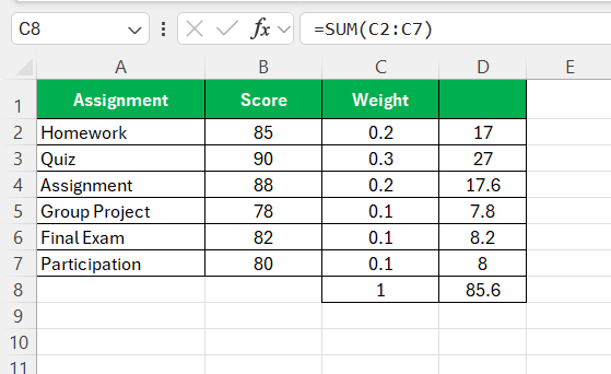
For instance, if I’m calculating my overall course grade, each assignment has a different impact on the final mark. Weighted average steps in to ensure that each score is given its appropriate significance. To put it simply, it’s the average accumulated not just by adding and dividing numbers, but by assigning importance to each number through weights.

This concept turns out to be crucial in fields such as education, finance, and data analysis, where emphasis on certain elements affects the outcome.

Excel and Its Formula Toolbox

Excel functions like a Swiss Army knife when it comes to number crunching, making my calculations swift and efficient. This is particularly true for weighted averages, where Excel’s formula toolbox comes into play. The formulas here are intricate tools, enabling us to not just perform basic arithmetic but also to manipulate and analyze data in sophisticated ways.

A standout feature of this toolbox is the set of functions specifically designed to handle different types of averages, including the indispensable SUMPRODUCT and SUM functions that are keystones for weighted average calculations. These functions allow for a multiplicity of operations – from the simplistic to the complex, making Excel a diligent workhorse in the arena of data analysis.

 

Mastering the Weighted Average Calculator in Excel

Laying the Groundwork: Entering Your Data Correctly

Before diving headfirst into the world of weighted averages, setting the stage with properly organized data is paramount. I’ve learned that Excel is unforgiving when it comes to incorrectly entered data, which can lead to flawed calculations and hours lost troubleshooting.

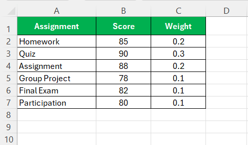
To prevent this, ensure that your data is clean and structured. Begin by designating separate columns for values (such as test scores or financial figures) and their corresponding weights (such as the percentage of the total grade or the share of investment in a portfolio). It’s also essential to avoid mixing data types within the same column, as Excel requires consistency to perform calculations correctly.

By meticulously entering data and paying close attention to detail, you’re setting yourself up for success when executing weighted average calculations, or indeed, any form of data manipulation in Excel.

Syntax of SUMPRODUCT

The basic structure is a formulaic translation of the concept of weighted average itself:

=SUMPRODUCT(range_of_values, range_of_weights) / SUM(range_of_weights)

By deconstructing the formula, it reveals a simple logic—each value is amplified by its weight through SUMPRODUCT, and then normalized by the weight’s collective sum. This ensures that the more significant items proportionally influence the result more than lesser ones.

Let’s dissect it component by component:

• SUMPRODUCT(range_of_values, range_of_weights) multiplies each value by its weight and then sums up these products.
• SUM(range_of_weights) computes the total weight, which serves as our divisor.

When deftly combined, these two functions embody the principle of weighted averaging in a sturdy, elegant computation.

The SUMPRODUCT Command: Your Key to Calculating Weighted Averages

The SUMPRODUCT function in Excel is quite the power player when it comes to weighted averages. It combines multiplication and addition, allowing me to multiply related data sets and sum up the results in one go. For those of you who appreciate efficiency, this command is a game-changer.

To use SUMPRODUCT for calculating weighted averages, two arrays are required: values and their corresponding weights. In Excel terms, arrays are simply ranges of cells. The magic happens when SUMPRODUCT multiplies each value in the first array with its corresponding weight in the second array and then sums it all up.

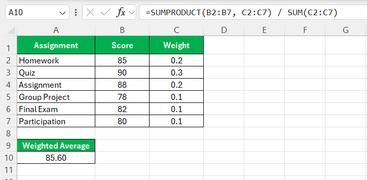
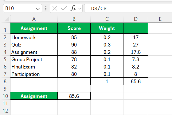
Here’s a practical formula structure: =SUMPRODUCT(B2:B7, C2:C7) / SUM(C2:C7)

This formula, where B2:B7 holds the values and C2:C7 holds the weights, simplifies the process, delivering the weighted average without the need for additional steps.

Alternative Routes: Using SUM and Helper Columns

Sometimes, clarity trumps conciseness. In scenarios where a transparent and easily traceable method is preferred, breaking the weighted average calculation into more digestible steps using SUM and helper columns is a prudent choice.

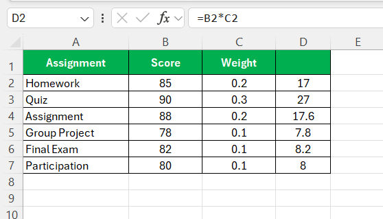
This alternate route involves creating an intermediary step: a helper column that multiplies each individual value by its corresponding weight. This creates a new array of weighted values which can then be summed using the SUM function to find the total sum of weighted values.

Next, to get the weighted average, I would divide the total sum of weighted values by the sum of the weights, also calculated using the SUM function on the weights array.

The formula might look like this:

STEP 1: In a third column, multiply each value by its weight: =B2*C2

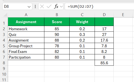
STEP 2: Sum the results of this column: =SUM(D2:D7) (with D2:D7 being the helper column)

STEP 3: Sum the weights: =SUM(C2:C7)

STEP 4: Divide the sum of the weighted values by the sum of the weights.

Though this method requires more space and a few extra steps, it greatly enhances the formula’s transparency and facilitates validation and error checking.

 

Deep Dive into Excel Formulas for Weighted Averages

Navigating Nonstandard Weights: When Totals Don’t Sum to One

Dealing with weights in Excel that don’t neatly sum up to one (or 100%) is a common occurrence, and it’s crucial to adjust the formula accordingly. It’s a flexible system: the sum of the weights can be any number, and Excel will manage just fine.

To navigate nonstandard weights, I adapt the formula slightly: =SUMPRODUCT(range_of_values, range_of_weights) / SUM(range_of_weights)

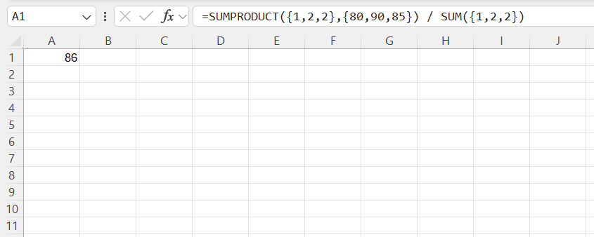
For example, if I had an array of weights that summed to 5 instead of 1, the formula would still hold true. The SUM function in the denominator does an excellent job of balancing out the equation, ensuring the weighted average remains accurate regardless of the total weight.

In practice, this looks like this: =SUMPRODUCT({1,2,2},{80,90,85}) / SUM({1,2,2})= (80*1 + 90*2 + 85*2) / 5= 430 / 5 = 86

Notice how the formula adjusts itself when the total weight changes. It’s just a matter of ensuring I divide by the correct sum of weights, and Excel does the rest.

 

Tips for Handling Large Datasets

When I’m working with a large dataset, the idea of manually calculating a weighted average can seem overwhelming. Here are a few tips I’ve found helpful:

• Use Named Ranges: Instead of manually selecting ranges each time, I like to name my ranges. For instance, I might name the score range Scores and the weight range Weights. This allows me to use those names directly in my formulas, like =SUMPRODUCT(Scores, Weights) / SUM(Weights). It’s a real timesaver!

• Dynamic Ranges: If my data frequently changes in size, I use Excel’s dynamic range capabilities. By converting my data into an Excel Table, the range automatically updates as I add or remove data. This is particularly useful when you’re dealing with evolving datasets.

 

Common Mistakes to Avoid

Over time, I’ve made my share of mistakes when calculating weighted averages in Excel. Here are a few common pitfalls I’ve learned to avoid:

• Not Normalizing Weights: Early on, I forgot that the weights should typically sum to 1. If they don’t, the final result can be misleading. If my weights add up to something other than 1, I normalize them by dividing each weight by the total sum of weights.
• Mixing Up Data: It’s easy to accidentally apply the wrong weight to the wrong value, especially when working with larger datasets. I always double-check that the weights correspond correctly to their respective values to avoid skewing my results.

 

FAQ: Tackling Your Weighted Average Challenges

How do you calculate the weighted average?

To calculate the weighted average, multiply each number by its weight, sum up these products, and divide the result by the sum of all weights. Use the formula =SUMPRODUCT(array_of_values, array_of_weights)/SUM(array_of_weights) in Excel to quickly compute it. This formula takes into account the varying significance of each item to provide a more accurate average.

What is the SUMPRODUCT in Excel?

SUMPRODUCT is an Excel function that multiplies corresponding components in given arrays, summing up the resulting products. Ideal for calculating weighted averages, it can handle single or multiple arrays and is often used in scenarios where different criteria need to be multiplied and then added together.

How Can I Calculate a Weighted Average Without SUMPRODUCT?

To calculate a weighted average without SUMPRODUCT, you can create a helper column to multiply each value by its weight, then use the SUM function to add these products. Finally, divide the sum by the total of the weights with another SUM function. The formula structure will look like =SUM(helper_column)/SUM(weights_column), giving you the same result with a more manual approach.

What Is the Formula for Weighted Average in Excel When Dealing with Percentages?

In Excel, when dealing with percentages, the weighted average formula is the same: =SUMPRODUCT(array_of_values, array_of_percentages)/SUM(array_of_percentages). Ensure that the percentages are in decimal format (e.g., 50% as 0.5) for accurate calculation. This formula ensures that each value is weighted by its percentage out of the total.

Can You Explain How to Use an Array Formula for Weighted Averages?

Certainly. To use an array formula for weighted averages, after typing your formula such as =SUM(weights*values)/SUM(weights), instead of pressing Enter, press Ctrl+Shift+Enter. Excel encases the formula in braces, indicating an array formula that processes multiple values at once. In newer Excel versions, just pressing Enter suffices due to dynamic arrays.