What is 20 of 40 in Excel: Quick Percentage of Number Formula Guide

Microsoft Excel, the computational wizard, demystifies the process of calculating percentages, transforming what seems like a daunting task into a straightforward and error-free procedure. By understanding percentages as fractions of 100 and utilizing Excel’s built-in formulas, users can quickly determine values such as what is 20 of 40, streamlining tasks like budget preparation, data analysis, and test grading.

Key Takeaways

• Percentages represent a part of a whole as a fraction of 100, simplifying the comparison and calculation of different quantities.
• Excel’s built-in formulas and percentage formatting options make percentage calculations swift, accurate, and visually clear, enhancing both efficiency and professionalism.
• The basic formula for calculating percentages in Excel is straightforward: =(Part/Total)*100, with Excel handling the multiplication by 100 automatically.
• Excel allows for easy percentage formatting either through ribbon options for quick application or the ‘Format Cells’ dialog box for customized displays, including the option to highlight negative percentages in red.

 

Unlock the Mystery of Percentages in Excel

Introduction to Percentage Calculations in Excel

Have you ever found yourself scratching your head wondering how to calculate something like “what is 20 of 40?” Especially when it comes to wrangling percentages. You’re not alone. Percentages can seem mysterious, but they’re a piece of cake with the right tools. Excel is that trusty sidekick that makes these calculations swift and painless.

Laying the Foundations: Percentage Basics

Understanding What Percentage Represents

Percentage can sometimes feel like a math puzzle where you’re juggling numbers in a cloud of confusion. But fret not, it’s much simpler than it seems. Think of a percentage as a way to express a number as a fraction of 100. If you picture a big pie cut into 100 slices, a percentage tells you how many of those slices you have. In your quest to figure out “what is 20 of 40,” you’re asking how big a slice of a 100-piece pie you’d have if 40 was the whole pie.

The Role of Excel in Simplifying Percentage Calculations

Excel shines as a computational wizard, turning the daunting task of percentage calculations into a walk in the park. You can bid farewell to the days of manual crunching of numbers with a calculator. Through its built-in formulas, Excel not only calculates percentages swiftly but also ensures accuracy every time you deal with data. Whether you are preparing a budget, analyzing data sets, or grading tests, Excel streamlines the process, saving you time and reducing errors.

 

Step-by-Step Guide to Calculate 20 of 40

Inputting Your Numbers Correctly

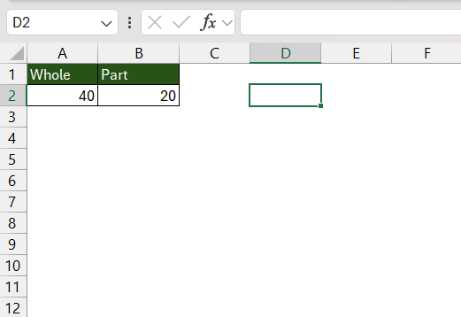
Before diving into the formula, getting the numbers right in Excel is crucial. Start by entering the number from which you want to calculate the percentage (in this case, 40) into a cell—let’s say A2. Then, in another cell B2, you’ll need to input the percentage you wish to calculate (20).

 

Using the Basic Excel Percentage Formula

To reveal the magic number — what 20 is of 40 in Excel — we will employ the basic Excel percentage formula. This formula is a breeze: =(Part/Total)*100. Here’s how you do it:

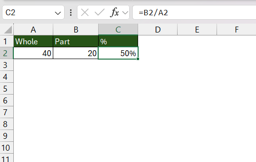
STEP 1: In your Excel worksheet, let’s assume cell A2 holds the total (40), and B2 holds the part (20).

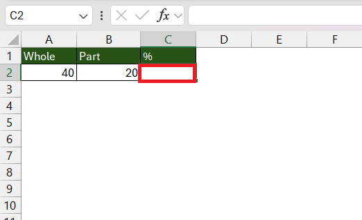
STEP 2: Click on an empty cell, say C2, where you want the result to appear.

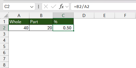
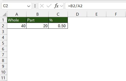
STEP 3: Type in the formula =B2/A2.

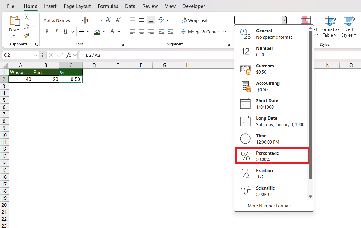
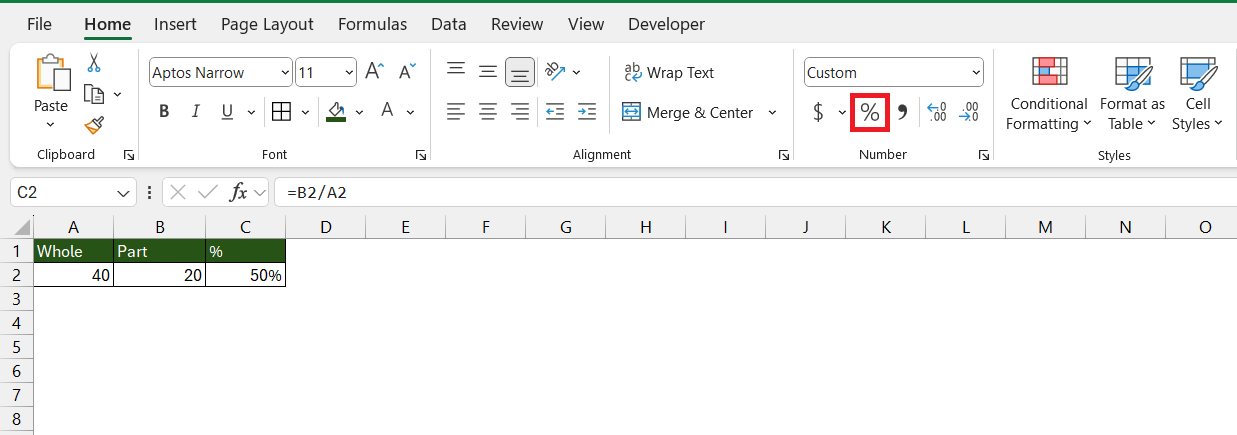
STEP 4: Then, apply percentage formatting: Select the cell with the result, go to the ‘Home’ tab, and under the ‘Number’ group, click on the percent symbol %.

Voila! Excel automatically multiplies by 100 and shows you the answer – it’s 50%.

Thus, 20 out of 40 is 50%, as accessible as a warm knife through butter with Excel doing the heavy lifting.

 

Visual Aids: Formatting Cells for Clearer Results

Method 1 – Applying Percentage Formatting via Ribbon Options

Excel offers a neat and swift way to transform your data into percentages using the ribbon options. Here’s how you glide through this process:

STEP 1: Select the cell or range of cells where you’ve performed your calculations.

STEP 2: On the Home tab, look for the ‘Number’ group.

STEP 3: Click on the Percentage Style button, a symbol with “%”, to instantly convert your selected numbers into percentages.

This one-click wonder not only saves time but adds professionalism to your data presentation, transforming 0.5 to 50% just like that.

 

Method 2 – Customizing Through the Format Cells Dialog Box

If you crave more control over how your percentages look, or if you’re using an older Excel version without the ribbon, the ‘Format Cells’ dialog box is your ticket to customization. Here’s the play-by-play:

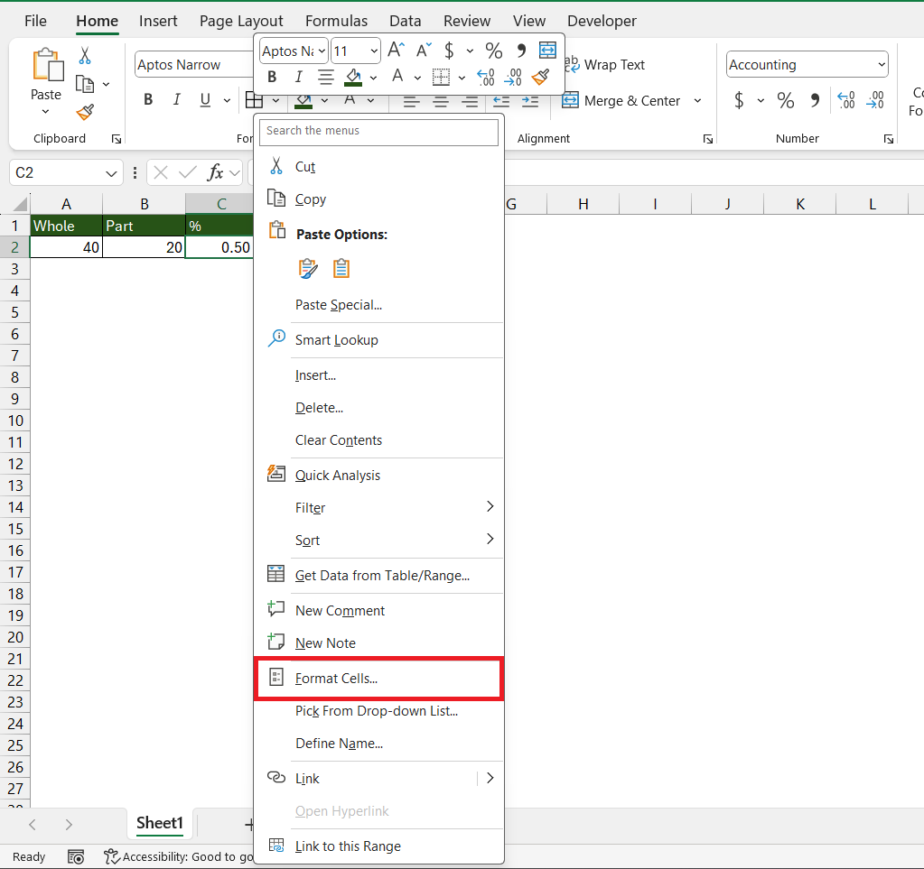
STEP 1: Highlight the cell(s) where you want to showcase a percentage.

STEP 2: Right-click and choose ‘Format Cells…’, or press Ctrl+1 for a keyboard shortcut to the dialog box.

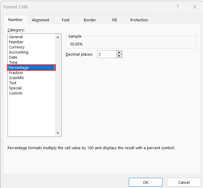
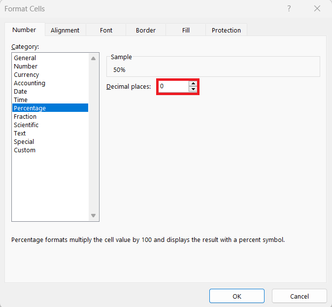
STEP 3: Click on the Number tab, then select ‘Percentage’.

STEP 4: For a precise display, pick the number of decimal places you fancy.

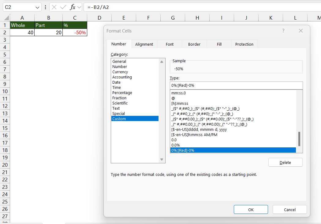
If it’s drama you’re after, you can set negative percentages to show up in red by choosing a Custom format like 0%;[Red]-0%.

After clicking OK, your cells will dress up in the formatting you picked out, and you’re set for the show.

 

Beyond the Basics: Adapting Formulas for Various Scenarios

Increasing a Number by a Percentage

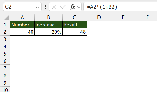
If your spreadsheet quest involves increasing a number by a percentage, you’re navigating familiar territory with Excel’s nifty formulae. Here’s how you conquer those calculations:

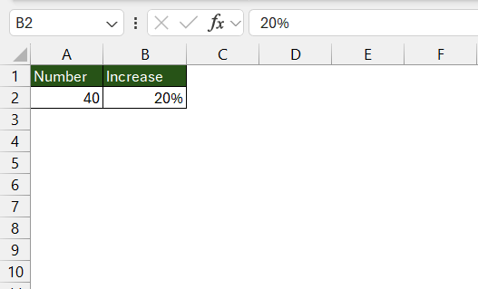
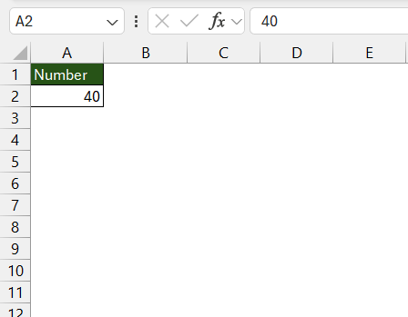
STEP 1: Place the original number in a cell (let’s call it cell A2).

STEP 2: Enter the percentage increase in another cell as a decimal (for instance, for 20%, you’d enter 0.20 in cell B2).

STEP 3: In a different cell, harness the power of Excel’s formula: =A2*(1+B2).

Excel enchants the original number, increasing it by 20% and displaying the new value right before your eyes.

This sorcery makes tasks like adjusting prices or calculating interest gains as easy as pie.

 

Figuring Out Percentage Decrease with Excel Formulas

Have you ever been in need to adjust numbers downward by a percentage? Maybe you’re calculating discounts or estimating expense reductions. Excel has got you covered yet again. Here’s the straightforward spell for lowering those figures:

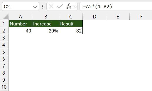
STEP 1: Start with the number you want to decrease in cell A2.

STEP 2: Next, jot down the percentage of the decrease as a decimal in cell B2. For example, a decrease of 20% would appear as 0.20.

STEP 3: Now, weave together the formula in cell C2: =A2*(1-B2).

With the charm of a formulaic wand wave, Excel shrinks the original number by the given percentage, presenting you with the lesser amount.

This formula ensures that whether you’re marking down prices or trimming a budget, Excel subtracts just the right amount of fairy dust from your figures.

FAQs: Your Questions, Answered

How do you calculate percentages using simple formulas?

To calculate percentages using simple formulas in Excel, enter the formula =(Part/Whole)*100 into a cell. Replace ‘Part’ with the cell reference of the part and ‘Whole’ with the cell reference of the whole. Excel will spit out the percentage value for you.

Can Excel automatically calculate percentage increases or decreases?

Yes, Excel can automatically calculate percentage increases or decreases. For an increase, use =Original_Number*(1+Percentage) and for a decrease, use =Original_Number*(1-Percentage), where ‘Percentage’ is the percentage change written in decimal form.

How do I calculate 20% of a number in Excel?

To calculate 20% of a number in Excel, you can use the formula `=number*0.2`, replacing “number” with the actual value you’re interested in. Alternatively, you could also use the formula `=20%*number`, and Excel will automatically interpret the 20% as 0.2 to perform the calculation.

How do you take 20% off a price in Excel?

To take 20% off a price in Excel, input the original price in a cell (e.g., A1), and in a neighboring cell, use the formula `=A1*(1-20%)`. Press ‘Enter’, and the cell will display the price after subtracting the 20% discount. If working with a list of prices, drag the fill handle down to apply this formula to the entire column.

How do you do 40% discount in Excel?

To apply a 40% discount in Excel, first ensure column A contains the original prices. Then, choose a blank cell where you will apply the formula =A2*(1-0.40) to calculate the discounted price. Press ‘Enter’ and drag the fill handle down to apply the 40% discount to all items listed. After the formula is applied, the cells will reflect the sale prices after a 40% reduction.