What’s Reference in Excel? Step by Step Cell Reference Guide

Excel, a powerful tool for data analysis and management, relies fundamentally on cell references to connect and calculate data. Understanding these references is crucial for creating efficient spreadsheets, allowing users to maintain consistency across datasets and ensuring their operations yield accurate results. This guide will walk you through the various aspects of cell references, unlocking their potential in Excel for enhanced spreadsheet utility.

Key Takeaways:

• Cell references in Excel allow formulas to retrieve and manipulate data dynamically.
• Relative, absolute, and mixed references control how cell addresses adjust when copied.
• The A1 and R1C1 styles offer different ways to identify cell locations in formulas.
• 3D references enable calculations across multiple worksheets for efficient data consolidation.
• Named ranges improve formula readability, while troubleshooting helps resolve common reference issues.

 

Understanding Excel Cell References

Defining Cell References

A cell reference in Excel is essentially an address that identifies a specific cell’s location within a worksheet. It usually consists of a column letter and a row number, such as A1 or B5. This address allows Excel to retrieve the data contained in that cell for use in formulas and other spreadsheet operations.

By using cell references, you can dynamically manipulate data, perform calculations, and create powerful analytical tools that update automatically as the data changes.

Purpose and Importance in Spreadsheet Management

Cell references serve a vital purpose in spreadsheet management by linking data points across the worksheet. They allow users to create dynamic formulas that automatically update when the source data changes, ensuring accuracy and efficiency in data processing.

Additionally, cell references reduce redundancy by avoiding manual data entry, therefore minimizing errors. Their importance is further underscored by their ability to facilitate complex calculations, support data analysis, and maintain the integrity of large datasets across multiple Excel sheets, enhancing overall productivity and decision-making.

 

Types of Cell References in Excel

Relative Cell References

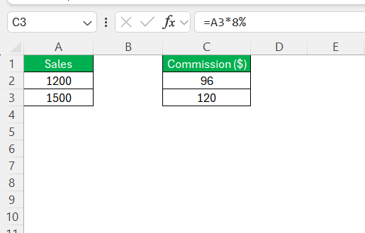
Relative cell references in Excel are references that adjust automatically when copied from one cell to another. They are denoted simply by the column letter and row number, such as A1. When you copy a formula containing relative cell references, Excel recalculates the formula for each new cell position, based on the original reference’s location.

For example, if you have a formula in cell C2 that references A2, and you copy it to C3, the reference will adjust to A3.

This dynamic feature makes relative references particularly useful for repetitive calculations across multiple rows or columns.

Absolute Cell References

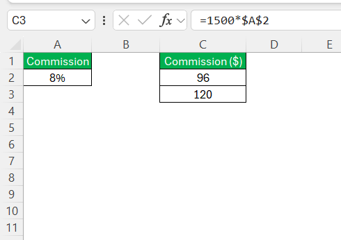
Absolute cell references in Excel remain constant, regardless of where they are copied in the worksheet. They are indicated by placing a dollar sign ($) before the column letter and row number, such as $A$1. This ensures that the reference points to the same specific cell, even when the formula is dragged or copied to other cells.

Absolute references are particularly beneficial when you need to apply a consistent, unchanging value across a range of calculations, such as using a fixed multiplier or a static constant in formulas. For example, to multiply values by a fixed tax rate in cell A2, the formula would look like =Value*$A$2 to maintain the reference to A2 consistently across multiple cells.

Mixed Cell References

Mixed cell references combine elements of both relative and absolute references, allowing either the column or the row to remain constant while the other component varies. This type of reference is denoted by a dollar sign ($) placed before either the column letter or the row number, such as $A1 or A$1.

They are particularly useful when working with data arrays and performing operations where either the column or the row needs to remain fixed as the formula is copied across other cells. For instance, if a formula is copied vertically and it should keep referencing the same column, you might use a mixed reference like $B2, ensuring that column B remains constant while the row number adjusts with each new position.

 

Mastering Reference Styles

A1 and R1C1 Reference Styles

Excel offers two primary reference styles: A1 and R1C1. The A1 reference style is the default and most commonly used format, where columns are labeled with letters (A, B, C) and rows with numbers (1, 2, 3). This format helps users easily identify cells through alphanumeric labels, such as C3 indicating column C, row 3.

On the other hand, the R1C1 reference style uses numbers for both rows and columns, where R refers to the row number and C to the column number. For example, R3C3 refers to the cell in the third row and third column. This style is particularly advantageous when writing macros, as it simplifies the process of identifying cell positions programmatically. Users can switch between these styles by adjusting the settings in Excel’s options, providing flexibility based on individual preferences or project requirements.

Using 3D References Across Multiple Worksheets

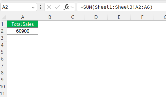
3D references in Excel allow you to reference the same cell or range of cells across multiple worksheets within the same workbook. This is particularly useful for consolidating data from similar sheets, such as monthly sales reports, into a singular calculation or summary. To create a 3D reference, start by typing your formula and selecting the first sheet you want to include. Hold the Shift key, click the last sheet tab you want to reference, and then select the cell or range on the last sheet. This action essentially forms a continuous range across the selected sheets.

For instance, the formula =SUM(Sheet1:Sheet3!A2:A6) would add up all the values from cells A2 to A6 across Sheet1, Sheet2, and Sheet3.

3D references streamline complex calculations that involve repetitive datasets in separate sheets, reducing manual data integration and ensuring consistency across analyses.

 

Advanced Techniques for Using Cell References

Creating References to Other Sheets and Workbooks

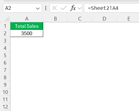
Creating references to cells in other sheets or workbooks allows you to build comprehensive spreadsheets that pull and utilize data from various sources seamlessly. To reference a cell in another sheet within the same workbook, use the sheet name followed by an exclamation mark before the cell address. For example, =Sheet2!A4 refers to cell A4 on Sheet2.

When referencing cells in another workbook, you’ll need to include the workbook name in square brackets, followed by the sheet name and the cell reference. Suppose you want to reference cell A1 in Sheet1 of a workbook named “Finance.xlsx.” The reference would look like this: =[Finance.xlsx]Sheet1!A1. If the workbook filename or sheet contains spaces or special characters, enclose it in single quotes, for example, ='[Annual Report.xlsx]Sheet1'!C2.

These techniques are powerful for building interconnected data models, maintaining data integrity across projects, and ensuring that your worksheets reflect the most current information from various data sets.

Converting References to Named Ranges

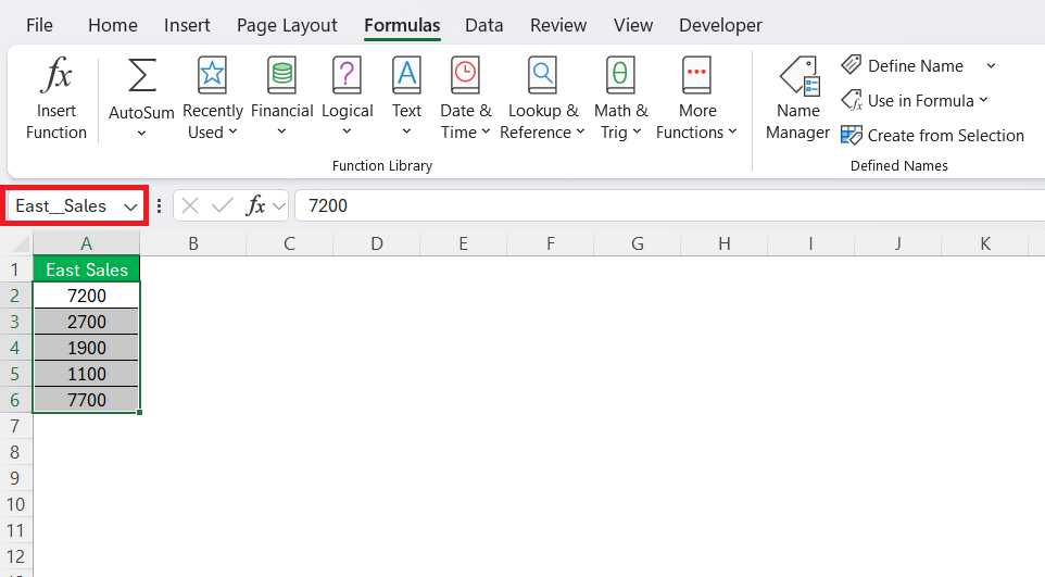
Converting cell references to named ranges in Excel enhances the readability and manageability of your spreadsheets significantly. Named ranges allow you to assign meaningful labels to individual cells or ranges, making formulas easier to understand. To convert references, select the cell or range you wish to name, enter a name in the Name Box (the field to the left of the formula bar), and press Enter. Names can include letters and numbers but must start with a letter.

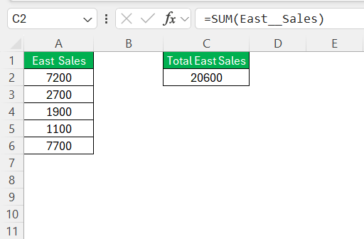
To implement named ranges in formulas, replace the cell reference with its defined name. For example, if you have named a range East_Sales, you could use it in a formula like =SUM(East_Sales) instead of specifying cell locations.

Named ranges not only make your formulas more intuitive, but they also ease navigation within large datasets, allowing for quick and error-free formula corrections whenever necessary. They are indispensable tools for maintaining clarity and consistency in complex Excel models.

 

Troubleshooting Common Issues

Resolving the F4 Shortcut Not Working

If the F4 shortcut key for toggling between relative and absolute references in Excel isn’t working, there could be a few potential causes and solutions. First, check if your keyboard requires the use of the Fn key to activate function keys; try pressing Fn + F4. If that doesn’t resolve the issue, the shortcut may be disabled, possibly overridden by another program capturing the F4 key. In this case, examine any existing shortcut configurations in your operating system or other software running concurrently with Excel.

Another step is to ensure you’re in formula edit mode—done by pressing F2 or double-clicking the cell containing the formula you wish to edit. If the problem persists, reviewing Excel settings for shortcut customization could help, or restarting Excel might reset any temporary glitches. These troubleshooting steps should restore the F4 functionality, enabling efficient toggling between reference types without manually typing dollar signs.

Handling Circular References

Circular references occur when a formula directly or indirectly refers back to its own cell. This can cause errors or infinite loops, disrupting the flow of calculations in Excel. To handle circular references effectively, start by identifying them; Excel typically displays an error message and highlights the circular reference cells. Navigate to Formulas > Error Checking > Circular References to locate all involved cells.

Once identified, you can resolve them by revising the formula to eliminate the self-reference. Sometimes, restructuring your spreadsheet model or using alternative formulas can help resolve the issue.

 

FAQs

What is a reference in Excel?

In Excel, a reference identifies a specific cell or range of cells within a worksheet. This allows users to include the values from those cells in formulas and functions, facilitating dynamic calculations and data management.

What is the difference between relative and absolute references?

Relative references in Excel adjust according to the formula’s new position when copied, while absolute references remain constant, always pointing to the same specific cell, regardless of where the formula is moved.

How can I use cell references across multiple workbooks?

To use cell references across multiple workbooks, include the workbook name in brackets, followed by the sheet name and cell address (e.g., =[WorkbookName.xlsx]Sheet1!A1). Ensure both workbooks are open, and use single quotes if the workbook or sheet names contain spaces.

What does the $ sign mean in Excel references?

In Excel, the $ sign in a cell reference designates that part of the reference as absolute. This means it won’t change when the formula is copied to another cell, ensuring the reference to a specific row or column remains constant.

What is cell address in Excel?

A cell address in Excel refers to the specific location of a cell in a worksheet, denoted by the combination of its column letter and row number, like A1 or B2. This address is used to identify the cell’s position for data entry and formula references.