2 Best Ways on How to Use XLOOKUP with Multiple Criteria

 

SYNTAX

To use the XLOOKUP function, you need to know the syntax and the parameters involved. The syntax of the XLOOKUP in Excel is:
=XLOOKUP(lookup_value,lookup_array,return_array,[if_not_found],[match_mode],[search_mode])

• Lookup_value: The value you want to search for.
• Lookup_array: The range of cells to search in.
• Return_array: The range of cells to return the result from.
• [if_not_found]: Value to return if no match is found. If left blank, no matches will return #N/A
• [match_mode]: The type of match to perform (exact or approximate). This is an optional parameter, and the default value is 0 (exact match).
  • 0 – Exact match. If none is found, return #N/A.
  • -1 – Exact match or return the next smaller item.
  • 1 – Exact match or return the next larger item.
  • 2 – A wildcard match : *, ?, and ~ have special meaning.
• [search_mode]: The direction of the search (left to right or right to left). This is an optional parameter, and the default value is 1 (left to right).
  • 1 – Perform a search starting at the first item.
  • -1 – Perform a reverse search starting at the last item.
  • 2 – Perform a binary search that relies on lookup_array being sorted in ascending order. If not sorted, invalid results will be returned.
  • -2 – Perform a binary search that relies on lookup_array being sorted in descending order. If not sorted, invalid results will be returned.

Now that you are familiar with the syntax of XLOOKUP, let us now explore how you can use XLOOKUP with multiple criteria.

• Method 1 – Boolean
• Method 2 – Concatenate

Make sure to download this Excel Workbook and follow along to understand how to use XLOOKUP with multiple criteria:

download excel workbookXLOOKUP-with-multiple-criteria.xlsx

 

METHOD 1 – BOOLEAN

XLOOKUP is especially preferred because of its ability to look up multiple criteria at once. The best way to do that is to use XLOOKUP with multiple criteria to use the Boolean logic. Now you might get confused by the name, but it is simply a complicated term for a simple condition – Either true or false.

In this example of XLOOKUP with multiple criteria, you want to get the price of a product that satisfies three conditions –

• Product Category is Pants
• Size is L
• Color is Blue

Let us go step by step with this formula!

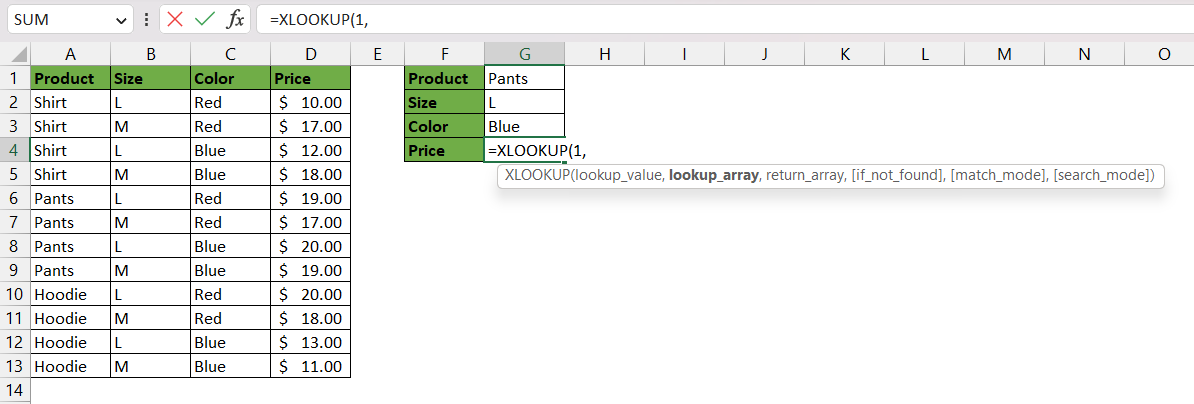
STEP 1: Enter the first argument – Lookup_value. Here our lookup value is 1. This is because test arrays will return 1 only when all the criteria are met.

=XLOOKUP(1,

STEP 2: Enter the second argument – Lookup_array. Here we are checking XLOOKUP with multiple criteria. We will call them our test arrays.

• First, the product category must be Pants. We are searching for matches of “Pants” in the entire array A2:A13.
• Second, the size should be L. We are searching for matches of “L” in the entire array B2:B13.
• Finally, the color should be Blue. We are searching for matches of “Blue” in the entire array C2:C13.

=XLOOKUP(1,(A2:A13=G1)*(B2:B13=G2)*(C2:C13=G3),

STEP 3: Enter the third argument – Return_array. Here we are going to select the entire array that contains all the prices i.e. D2:B13.

=XLOOKUP(1,(A2:A13=G1)*(B2:B13=G2)*(C2:C13=G3),D2:D13)

Here we are creating a list of arguments that we want to fulfill in our search. We are looking for an exact match by using the “=” operator.

=XLOOKUP(1,(A2:A13=G1)*(B2:B13=G2)*(C2:C13=G3),D2:D13)

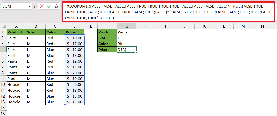
The test arrays will return TRUE or FALSE as a result, where TRUE indicates that the condition has been met and similarly, FALSE means the condition has not been met.

=XLOOKUP(1,{FALSE;FALSE;FALSE;FALSE;TRUE;TRUE;TRUE;TRUE;FALSE;FALSE;FALSE;FALSE}*{TRUE;FALSE;TRUE;FALSE;TRUE;FALSE;TRUE;FALSE;TRUE;FALSE;TRUE;FALSE}*{FALSE;FALSE;TRUE;TRUE;FALSE;FALSE;TRUE;TRUE;FALSE;FALSE;TRUE;TRUE},D2:D13)

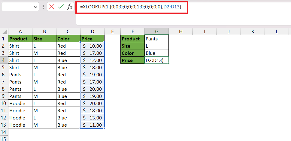
The multiplication operator will convert the TRUE and FALSE to 1s and 0s.

=XLOOKUP(1,{0;0;0;0;0;0;1;0;0;0;0;0},D2:D13)

We can see this in a more straightforward way also.

Cell G1 contains the product category you want to look up in the array A2:A13. What the function will do is search for “Pants” in every row of the array selected. It will then return the value 1 for every row where it finds a match, and 0 for no matches.

Similarly, you enter arguments to search the required Size (mentioned in cell G2) and Color (mentioned in cell G3) in the corresponding columns B2:B13 and C2:C13.

Finally, we are multiplying each argument using the “*” operator. This will ensure that the only row that returns a value of 1, meets all the required criteria.

In the result, you can see that only Row 7 has TRUE matches in three columns (Lookup arrays), hence it has returned the value 1. When multiplying, only Row 7 will return the value 1, as all others will have at least one 0 in their formula, making the end result 0 as well.

 

METHOD 2 – CONCATENATION

When using boolean logic, you are testing different criteria and using TRUE or FALSE results to extract the required value. Instead, you can simply concatenate or join our lookup values and the lookup arrays to search for multiple criteria at once.

You can use the Ampersand (&) sign for concatenation. The & sign works as a concatenation operator and clues together texts for different cells.

Click here to learn three different ways to concatenate in Excel!

 

Let us work on the same example and see how to use & sign and get XLOOKUP with multiple criteria to work.

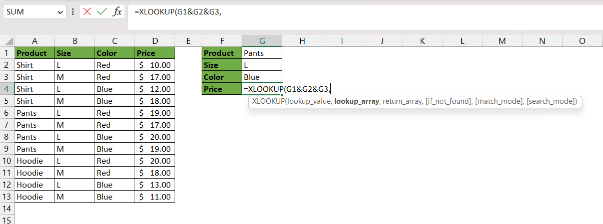
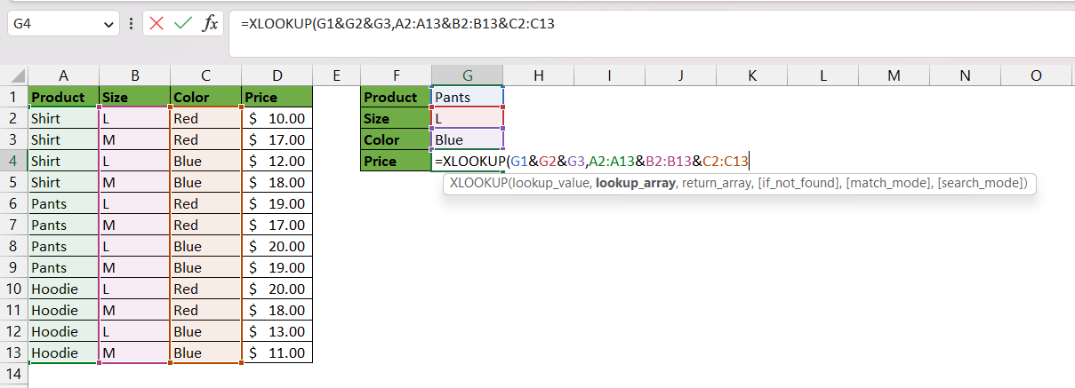
STEP 1: Enter the first argument – Lookup_value. Here our lookup value is the concatenation of the three conditions mentioned in cells G1, G2, and G3.1.

=XLOOKUP(G1&G2&G3,

Here we have clubbed all the criteria that we want to look up. Our three criteria are in the cells G3, G4, and G5, namely Product type, size, and color. Using the “&” operator, we have clubbed the cells together to look up these values simultaneously.

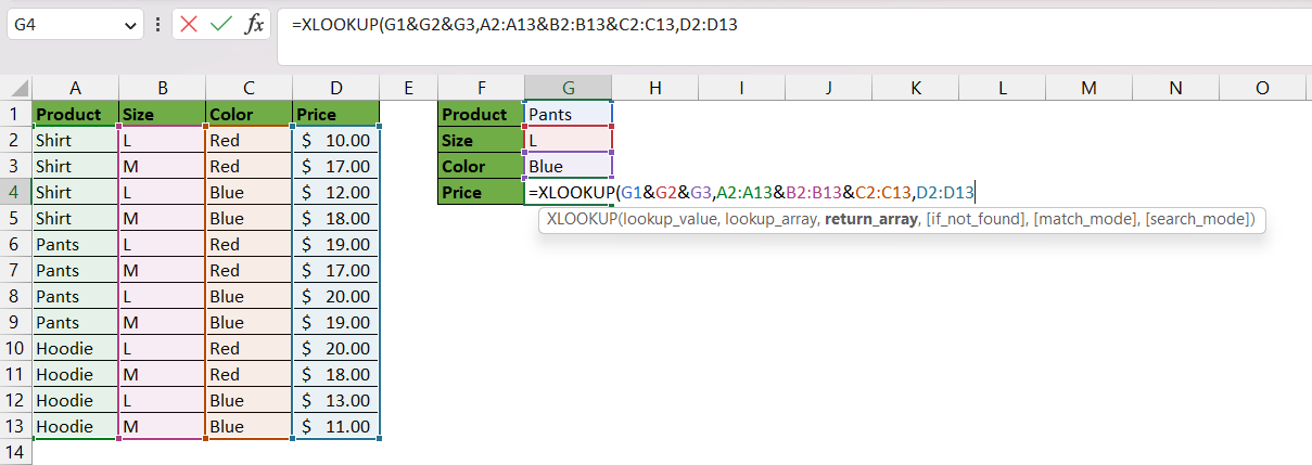
STEP 2: Enter the second argument – Lookup_array.

=XLOOKUP(G1&G2&G3,A2:A13&B2:B13&C2:C13,

We have similarly clubbed the corresponding lookup arrays for Product Category, Size, and Color using the “&” operator. Make sure to maintain the sequence of lookup values and corresponding lookup arrays.

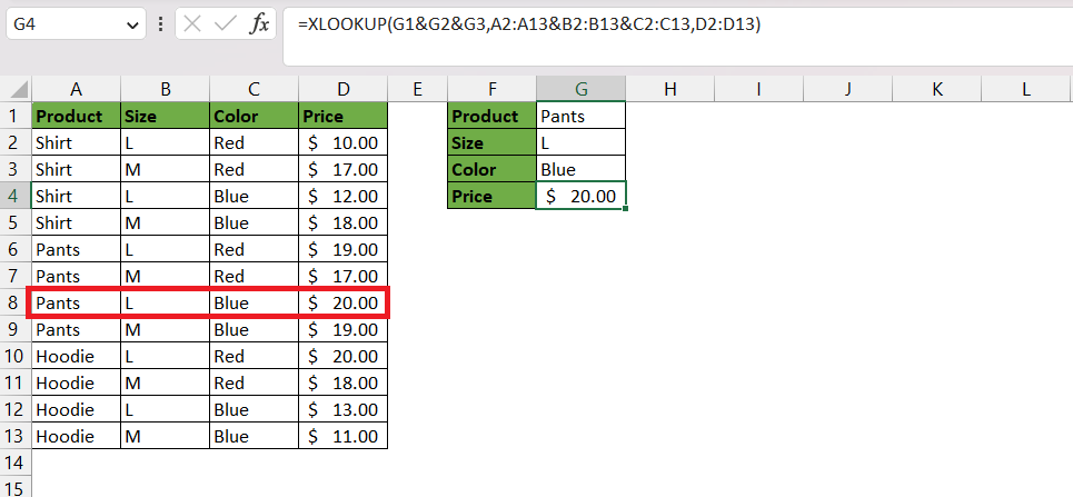
STEP 3: Enter the third argument – Return_array. Finally, we have selected the Price column D2:D13 as we want to extract the price of the product.

=XLOOKUP(G3&G4&G5,A2:A13&B2:B13&C2:C13,D2:D13)

Using the & sign, you can easily use XLOOKUP with multiple criteria and get the desired result.

 

Conclusion

You can either use Boolen or & sign to use XLOOKUP with multiple criteria in Excel. The concatenation approach may be easier to use, but the Boolean logic is far more flexible and powerful. You can decide which method to use based on its application and requirement.

Please Note – XLOOKUP is available for Microsoft 365 users only. So, make sure to upgrade your account to use XLOOKUP with multiple criteria.

Click here to learn how to use XLOOKUP in Excel using 11 different examples and applications.