Excel XMATCH Function – The Ultimate Guide with Examples

XMATCH in Microsoft Excel revolutionizes data search and analysis, offering a dynamic upgrade from the traditional MATCH function. Its introduction in Excel 2021 provides users with enhanced capabilities for complex data manipulations, enabling precise and efficient lookups in both one-dimensional and multidimensional arrays.

5 Key Takeaways:

• XMATCH offers a versatile syntax with optional arguments for match and search modes, accommodating exact, greater-than, less-than, and wildcard matches.
• It introduces significant improvements over MATCH, including reverse search capabilities and binary search options for sorted arrays, enhancing data navigation and analysis.
• By combining XMATCH with INDEX, users can perform powerful 2D searches across rows and columns, facilitating advanced data retrieval strategies.
• The function’s compatibility with wildcards (* and ?) extends its utility in managing varied data entries, making it invaluable for partial match searches.
• XMATCH’s introduction addresses the limitations of previous Excel lookup functions, positioning it as a superior choice for modern data processing tasks, with added benefits like default exact matches and support for unsorted data.

 

Introducing XMATCH: The Excel Pro’s Dynamic Tool

What is XMATCH in Excel?

XMATCH in Excel is a versatile lookup function that allows you to search for a specific item in a range or array and return the relative position of the item. With its introduction in Excel 2021, XMATCH has become a favorite tool for Excel aficionados looking to efficiently navigate through data. It is especially useful for comparisons, searches, and indexing within both one-dimensional and multidimensional ranges.

The Evolution from MATCH to XMATCH

The transition from MATCH to XMATCH in Excel marks a significant upgrade in lookup functionality. Initially, MATCH provided users with basic lookup capabilities, but with increasing demand for more complex data manipulation, the limitations became apparent. XMATCH was developed to address these gaps by incorporating enhanced features such as defaulting to an exact match, reverse searches, and enabling binary searches—offering a more dynamic experience for heavy Excel users.

 

Core Concepts of XMATCH Functionality

Understanding XMATCH Syntax and Arguments

The XMATCH function in Excel boasts a simple yet powerful syntax, allowing for diverse searching options. The structure of XMATCH goes as follows:

=XMATCH(lookup_value, lookup_array, [match_mode], [search_mode])

Here’s a breakdown of what each argument signifies:

• Lookup value (required): The data you want to find. It can be text, numbers, or wildcards like * and ?.
• Lookup array (required): The array or range where the search will take place.
• Match mode (optional): Determines the nature of the match. If omitted, it defaults to 0 for an exact match. You can specify -1 or 1 for less-than/greater-than matches and 2 for wildcard use.
• Search mode (optional): Defines the direction and method of the search. Leaving it out defaults to a search from the first item, but you can opt for -1 to start from the end or use binary search options (2 or -2) for sorted arrays.

Understanding these parameters equips you with the versatility to execute a range of searches tailored to your specific data analysis needs.

Match Type: Decoding the Four Unique Modes

XMATCH further empowers Excel users by offering four distinct match modes, greatly expanding the flexibility of data lookup tasks. Let’s decode these unique modes:

1. Exact Match (0 or omitted): When you desire an exact match for your lookup value, this is your default go-to mode. The function returns an #N/A error if no exact match is found.
2. Exact Match or Next Smaller Item (-1): If an exact match isn’t found, this mode instructs XMATCH to return the next smaller item relative to the lookup value.
3. Exact Match or Next Larger Item (1): In contrast to the previous mode, this one yields the next larger item when an exact match is not available.
4. Wildcard Match (2): This special mode enables the use of wildcard characters (* for multiple characters and ? for single characters), allowing partial match searches that can be particularly handy for text data.

Utilizing these match types correctly will enable succinct and powerful data query possibilities in your spreadsheets, ensuring you match the right data point every time.

 

Mastering XMATCH Examples and Scenarios

Example #1: Basic Usage for Single-Dimension Lookups

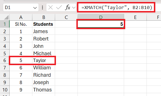
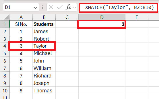
In single-dimension lookups, XMATCH shines by finding positions within a single row or column. Suppose you want to identify the position of a specific salesperson in a vertical list.

=XMATCH("Taylor", B2:B10)

Here’s what happens:

• Lookup value: “Taylor”
• Lookup array: B2:B10
• You’re essentially asking, “Where does Taylor appear in the list from A2 to A10?”

The function searches the range and returns Taylor’s position relative to the array’s start point. So, if Taylor is listed in cell B4, XMATCH would return 3 since Taylor is the third item from the top (starting at B2).

This basic usage can be a game-changer when dealing with tasks like creating dynamic charts or verifying data entry positions.

 

Example #2: Combining XMATCH with INDEX for 2D Searches

When the data spans across both rows and columns, pairing XMATCH with the INDEX function can effectively transform your 1D searches into a 2D data discovery journey.

Here’s an example formula:

=INDEX(return_array, XMATCH(lookup_value, lookup_array))

Imagine you’re seeking the sales figures for a specific month and salesperson. You would use:

• Return array: The range encompassing the monthly sales data.
• Lookup value: The name of the salesperson or the month you are searching for.
• Lookup array: The row or column containing the salesperson names or months.

For instance, to find the sales for a salesperson named Alex in March, the formula would be:

=INDEX(B2:M5, XMATCH("Taylor", A2:A5), XMATCH("March", B1:M1))

• First XMATCH: Searches for “Taylor” vertically in the list of salespeople.
• Second XMATCH: Searches for “March” horizontally in the list of months.

The INDEX function then retrieves the intersecting value where the salesperson’s row meets the month’s column—Taylor’s sales in March.

This powerful combination enhances your data analysis capabilities by providing precise values from multi-dimensional tables without resorting to complex, nested functions.

Advanced Tips and Tricks for Using XMATCH

XMATCH Reverse Search: Revealing Hidden Insights

One of the standout features of XMATCH is its ability to perform a reverse search, revealing hidden insights by searching from the end of the array towards the beginning. This capability is particularly useful when you need to find recent occurrences or the last match of a specific value within a dataset.

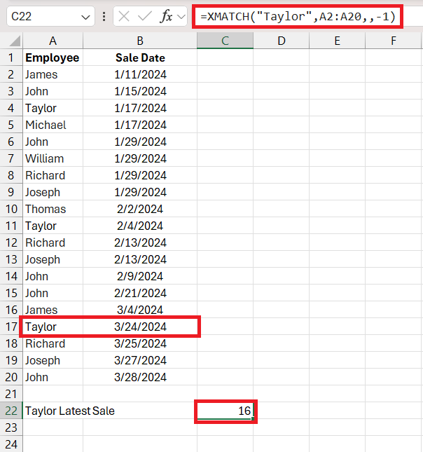
To execute a reverse search, set the optional search mode argument to -1, like this:

=XMATCH(lookup_value, lookup_array, , -1)

Let’s consider you have time-stamped data entries, and you want to find the last recorded instance of a particular event:

• Lookup value: The event you’re interested in.
• Lookup array: The range of time-stamped events.
• Search mode: -1 signifies the function should search in reverse.

Suppose you need to find the last sale made by a particular employee before the end of the record. By doing the reverse search, XMATCH will scan from the end of the list to return the position of the last occurrence of that employee’s sale.

This reverse search feature greatly enhances your ability to understand trends over time or pinpoint the most recent data points in a chronological dataset.

 

Utilizing Wildcards for Flexible Matching

The flexibility of XMATCH is further bolstered by its ability to utilize wildcards for matching patterns that are not exactly the same as the search term, which is incredibly powerful when dealing with data variations. The asterisk (*) and question mark (?) serve as the wildcard characters, allowing for partial matches.

Wildcard Usage:

• The asterisk * represents any series of characters.
• The question mark ? represents any single character.

Here’s how to conduct a wildcard search with XMATCH:

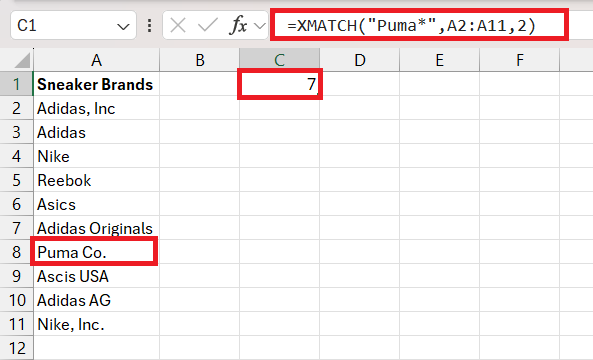
=XMATCH("Puma*", A2:A10, 2)

In this scenario, you’re telling Excel to locate the first instance of a phrase that begins with “Puma” and can be followed by any sequence of characters, as denoted by the asterisk *. With the match_mode set to 2, XMATCH treats the asterisk as a wildcard rather than a literal character.

For example, this allows you to find “Puma Co.” in a list even if you just search for “Puma”. The wildcard tells XMATCH to ignore anything after “Puma”, so it matches “Puma Co.” without a hitch, even though it isn’t an exact match.

Wildcards make XMATCH a potent tool for sifting through variations in data, such as different naming conventions or partially completed entries, facilitating a broader and more adaptable data search.

Note on Special Characters: If your search includes special characters that are normally treated as wildcards (like * or ?), XMATCH will treat them as literal characters without needing additional notation, ensuring accurate searches regardless of character type.

 

Common Hurdles: Troubleshooting XMATCH Errors

Handling Errors: Preventing Common XMATCH Pitfalls

Encountering errors while using the XMATCH function can be a pesky hurdle, but understanding how to troubleshoot can save you time and frustration. Here’s how to prevent some common XMATCH pitfalls:

• Ensure range consistency: The lookup_array should be a single row or column for XMATCH to work properly. Mixing row and column ranges can lead to unexpected errors.
• Verify data types: Mismatches between data types, such as numbers formatted as text, can prevent correct matching. Confirm that the lookup_value and lookup_array data types align.
• Use appropriate match mode: Choosing the correct match mode is vital, as the default mode (0) only works for exact matches. If an approximate match is required, use -1 or 1 accordingly.
• Beware of sorted requirements: Binary search modes (2 or -2) require a sorted lookup_array. Using these modes without sorting your data first can yield incorrect results.
• Handle #N/A errors: An #N/A error means no match was found. To gracefully handle this, combine XMATCH with the IFNA function:
• =IFNA(XMATCH(lookup_value, lookup_array), "Not Found")
• This setup replaces the #N/A error with a custom message, enhancing the readability of the results.

By preemptively preventing these errors, you’ll increase the efficiency and reliability of your Excel workbooks, ensuring that your data analysis is both accurate and insightful.

 

Assessing Alternatives When XMATCH Doesn’t Fit the Bill

In some instances, XMATCH might not be the best tool for your specific Excel task. If you find that XMATCH is not serving your needs, consider the following alternatives:

1. XLOOKUP: This function is a comprehensive solution that replaces VLOOKUP and HLOOKUP by returning the corresponding value, not just the position. XLOOKUP is perfect for direct retrieval of items.
2. VLOOKUP/HLOOKUP: If you’re using an older Excel version that doesn’t support XMATCH, these functions might come in handy despite their limitations compared to XMATCH and XLOOKUP.
3. INDEX and MATCH combo: It’s a classic pair that can mimic XMATCH capabilities by locating a value within a two-dimensional range. It offers a legacy approach for versions without XMATCH.
4. FILTER and UNIQUE functions: These dynamic array functions are helpful when you want to retrieve multiple matches or create unique lists dynamically.

Each function or combination addresses different needs. Consider the complexity of the task, the Excel version you’re working with, and the specific goal you want to achieve when deciding whether to use XMATCH or another alternative.

 

XMATCH Versus Other Lookup Functions

Why Choose XMATCH Over VLOOKUP or HLOOKUP?

Choosing XMATCH over VLOOKUP or HLOOKUP comes down to flexibility and control:

1. Default to Exact Matches: Unlike VLOOKUP’s default behavior of an approximate match, XMATCH defaults to an exact match, reducing unintended results.
2. Versatility in Search Direction: XMATCH can search from the top or bottom, while VLOOKUP and HLOOKUP are directionally fixed (downward and rightward, respectively).
3. Dynamic Arrays Compatibility: With Excel’s dynamic arrays capability, XMATCH integrates seamlessly, while VLOOKUP and HLOOKUP may require more workarounds.
4. Simplified Handling of Match Types: XMATCH offers a more intuitive approach to controlling match behavior with its match mode argument.
5. Unsorted Data Searches: Finally, XMATCH doesn’t require the lookup array to be sorted for approximate matches, which is a significant advantage over VLOOKUP and HLOOKUP, offering increased accuracy and speed in unsorted datasets.

Why XMATCH stands out:

• XMATCH provides additional match modes such as reverse searches and wildcard support, which are not available with VLOOKUP/HLOOKUP.
• It requires fewer arguments for a more straightforward formula.

XMATCH is a modern, versatile, and robust alternative tailored for a broader range of lookup tasks in Excel.

 

Performance Showdown: XMATCH vs. MATCH Functions

When it comes to choosing between XMATCH and MATCH in Excel, performance is a key factor. Here’s how they compare:

1. Match Modes: While MATCH supports approximate and exact matches, XMATCH adds the ability to search for the next larger or smaller item, giving users a finer degree of control.
2. Search Direction: MATCH searches in one direction—XMATCH steps up with the option to perform reverse searches, adding a layer of convenience when navigating through data.
3. Sorted Data: Unlike MATCH, XMATCH does not require data to be sorted for approximate match searches. This means you can use XMATCH in more scenarios without preliminary data sorting.
4. Binary Search: For sorted arrays, XMATCH can employ a binary search that’s optimized for speed, aiding in quicker lookups.
5. Enhanced Wildcard Functionality: XMATCH accepts wildcards for partial matches, something MATCH can’t accommodate directly.

While both functions have their merits, XMATCH delivers a more robust set of features, including improved error handling, making it the better choice for complex and varied datasets.

 

FAQs: Answering Your Lingering XMATCH Queries

How do you use Xmatch in Excel?

To use XMATCH in Excel, input the function followed by the item you’re searching for and the range where it should look. For a basic match, the formula is:

=XMATCH(lookup_value, lookup_array)

Customize with optional match_mode and search_mode to refine your search.

Can XMATCH Be Used with Conditional Arrays?

Absolutely! XMATCH can be used with conditional arrays, enhancing the ability to perform lookups based on specific criteria within Excel.

How Does XMATCH Behave with Partial Matches and Wildcards?

XMATCH handles partial matches using wildcards like * for any number of characters and ? for a single character. Set match_mode to 2 for this flexibility.

Is XMATCH Available in All Versions of Excel?

No, XMATCH is only available in Excel for Microsoft 365 and Excel 2021. Older versions do not support this function.

What is the difference between Xmatch and match?

XMATCH is more advanced with default exact match, reverse search capabilities, and support for unsorted data, unlike the older MATCH function.

What is the difference between Xlookup and Xmatch?

XLOOKUP retrieves the value corresponding to a match, while XMATCH provides the relative position of the match within a range. XLOOKUP is more a direct replacement for VLOOKUP/HLOOKUP, whereas XMATCH replaces MATCH, offering position-based lookups and is often used together with INDEX to pull values from a table.