A ratio is a mathematical concept representing the relationship between two or more quantities. The basic form of ratio is a/b and it is often written as a:b. In this article, we’ll explore four methods to calculate ratios using Excel functions –
Table of Contents
Let us look at each of these methods in detail.
Download the Excel Workbook below to follow along and understand How to Calculate Ratio in Excel –
download excel workbookCalculate-Ratio-in-Excel.xlsx
Method 1 – Simple Division
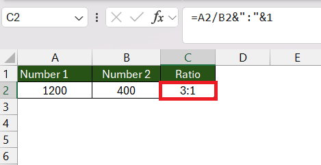
This method is useful when the larger number is completely divisible by the smaller number. Suppose, you have two numbers 1200 and 400 and you want to display them in the ratio format i.e. a:b.
You can first divide the two numbers using the division (“/”) sign and then use the & sign to add the colon. Next, you can add 1 after the colon sign.
The formula for this method is –
=A2/B2&”:”&1
Follow the steps below to use a simple division method to calculate ratio –
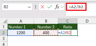
STEP 1: Divide the two numbers in cell C2.
=A2/B2
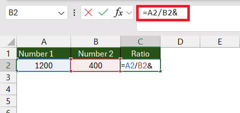
STEP 2: Enter the & sign.
=A2/B2&
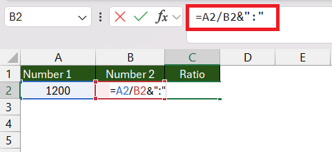
STEP 3: Enter the colon sign within quotes.
=A2/B2&”:”
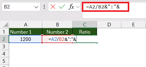
STEP 4: Enter the & sign.
=A2/B2&”:”&
STEP 5: Type 1.
=A2/B2&”:”&1
The result is 3:1.
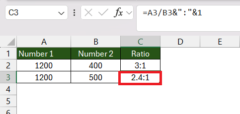
This method is not helpful if the numbers are not divisible and leave a remainder. If we divide 1200 by 500, the result will be displayed in decimal format as shown below.
You can use the other methods in this article to work on when encountered with such scenarios.
Method 2 – GCD Function
GCD is the function that returns the greatest common divisor of two or more integers. It is the largest integer that divides both numbers without a reminder. The syntax of this function is –
=GCD(number1, [number2], …)
where,
- number1 – The first number. Required.
- number2 – The second number. Optional.
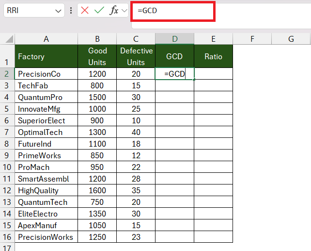
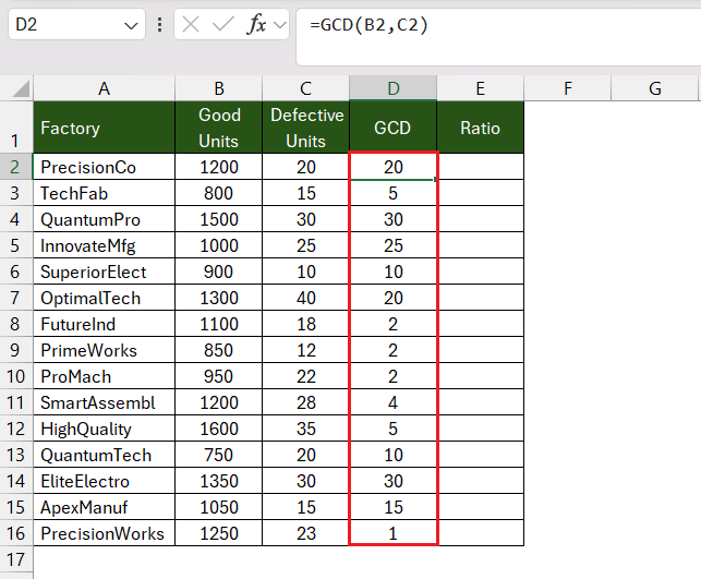
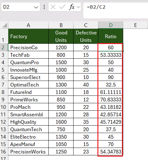
Imagine you have data on the production output of different factories in terms of units produced and the number of defective units, and you want to calculate the ratio of good units to defective units.
The objective is to ascertain the GCD between these two integers and subsequently utilize it to determine the ratio. Follow the steps below to calculate ratio in Excel –
STEP 1: Enter the GCD formula in cell D2.
=GCD
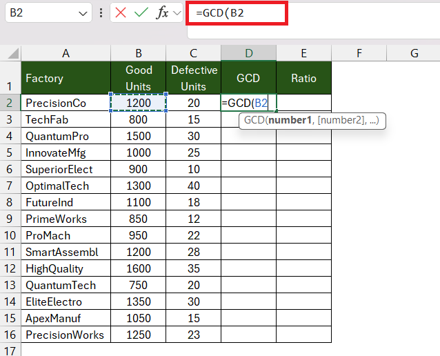
STEP 2: Select the first number mentioned in cell B2.
=GCD(B2,
STEP 3: Select the second number mentioned in cell C2.
=GCD(B2,C2)
STEP 4: Press Ctrl + D to copy the formula down.
This will provide you with the largest integer that divides both numbers without leaving a reminder.
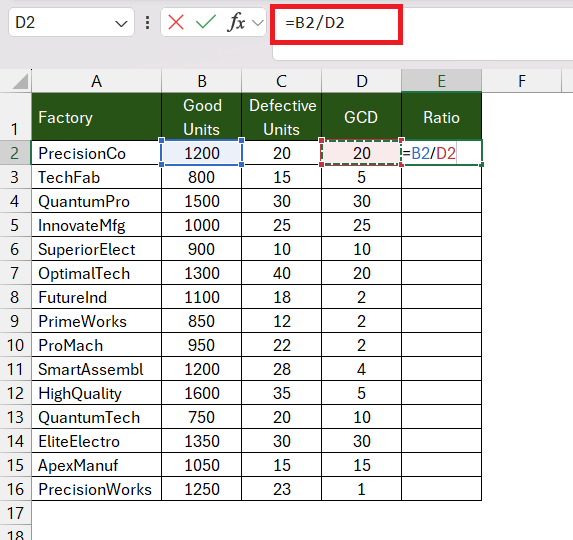
STEP 4: Divide the first number with GCD (calculated in cell D2).
=B2/D2
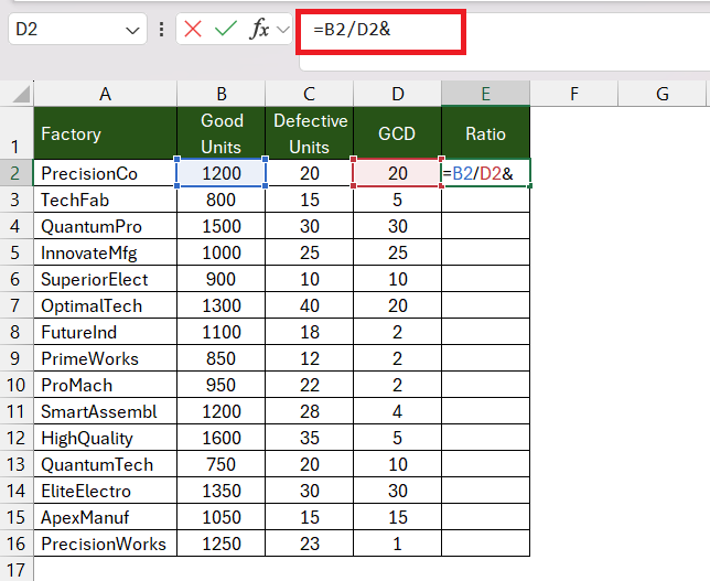
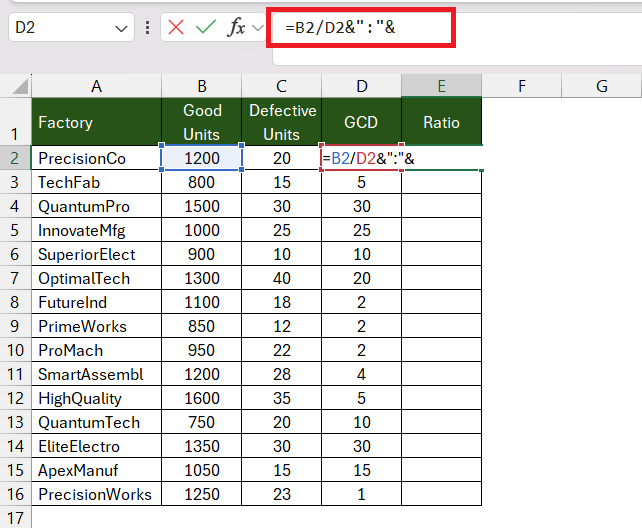
STEP 5: Enter the & sign.
=B2/D2&
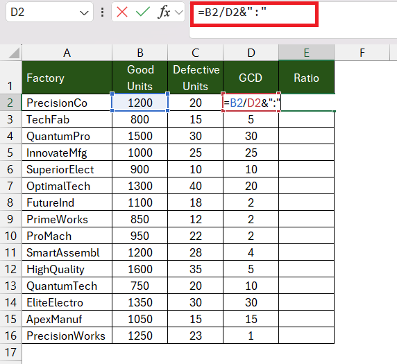
STEP 6: Enter the colon sign within quotes.
=B2/D2&”:”
STEP 7: Enter the & sign.
=B2/D2&”:”&
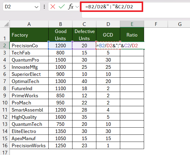
STEP 8: Divide the second number with GCD (calculated in cell D2).
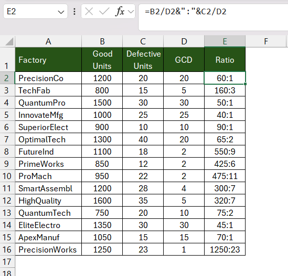
=B2/D2&”:”&C2/D2
The ratios will be displayed in column E. This is a quick and easy way to calculate ratios in Excel.
Method 3 – Custom Format
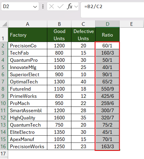
You can easily use the custom format option available in Excel to simply divide the two numbers and display the result in the format of a fraction i.e. a/b. The only issue with this method is that you can display the result with the separator as a forward slash only.
Follow the steps below to calculate ratio in Excel using the custom format –
STEP 1: Divide the two numbers in cell D2.
STEP 2: Press Ctrl + D to copy the formula down.
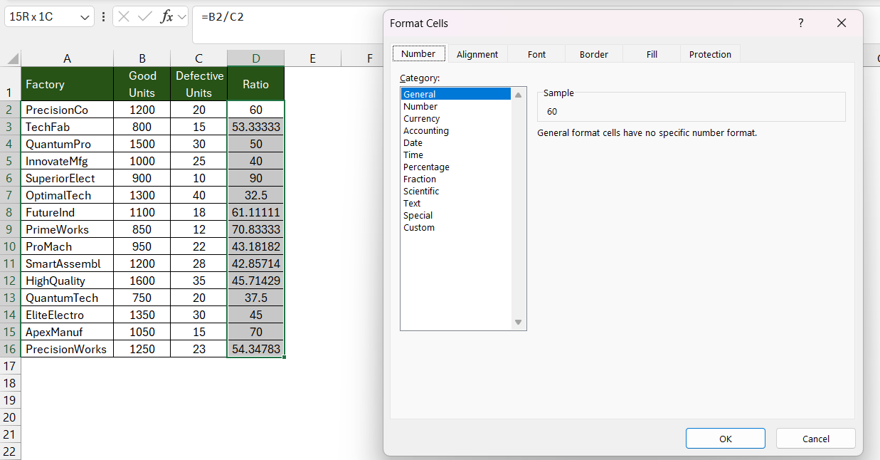
STEP 3: Select the range and press Ctrl+1 to open the Format Cells dialog.
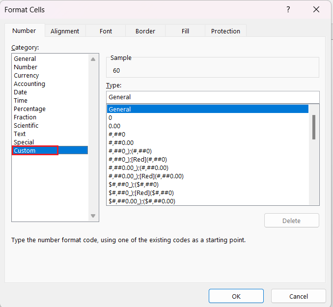
STEP 4: Under the Number tab, choose the Custom option.
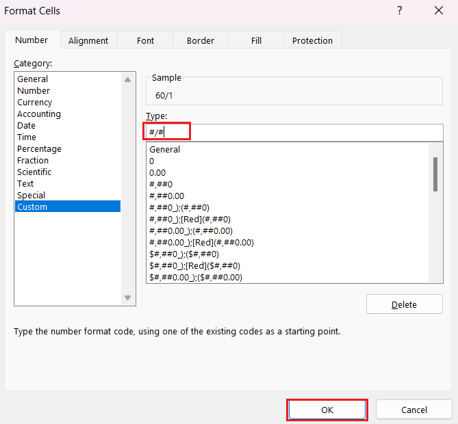
STEP 5: Type the Ratio format (“#/#”). Then Press OK.
The custom format i.e. a/b will be displayed in the range.
But, if you wish to display the ratio in the format a:b, you need to follow the next method.
Method 4 – TEXT & SUBSTITUTE Function
Another method to calculate ratio in Excel is to use a combination of TEXT and SUBSTITUTE functions. You need to first divide the two numbers and then use the TEXT function to display the decimal as a fraction. This fraction can be replaced from a/b format to a:b format using the SUBSTITUTE function.
The formula for this method is –
=SUBSTITUTE(TEXT(Num1/Num2, “#/######”),”/”,”:”)
Follow the steps below to achieve this result –
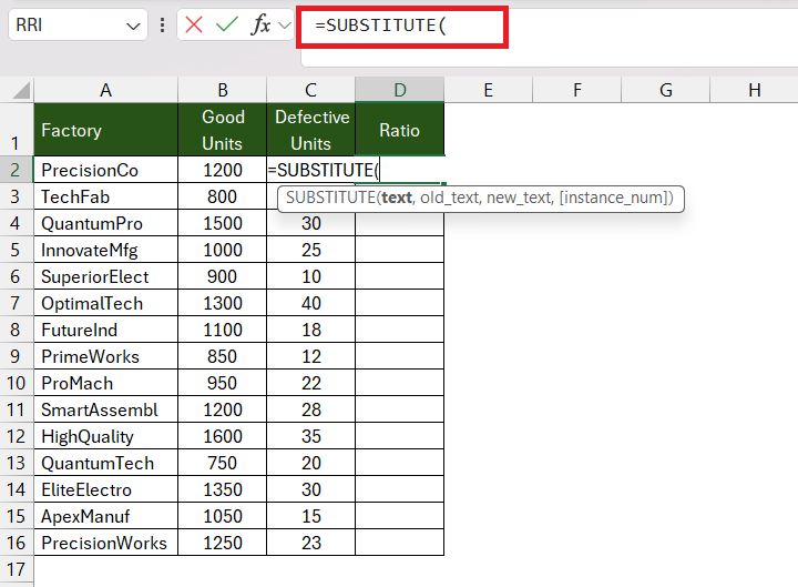
STEP 1: Enter the SUBSTITUTE function.
=SUBSTITUTE
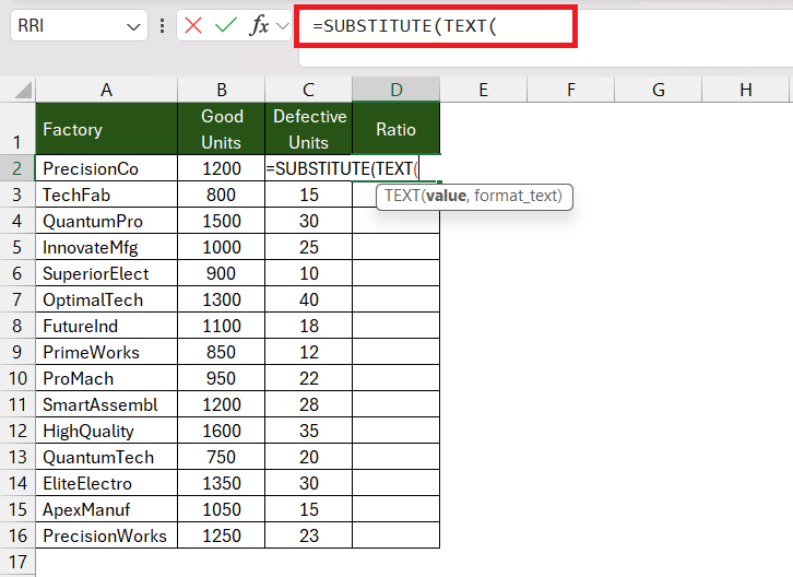
STEP 2: Enter the TEXT function.
=SUBSTITUTE(TEXT
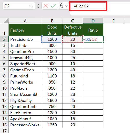
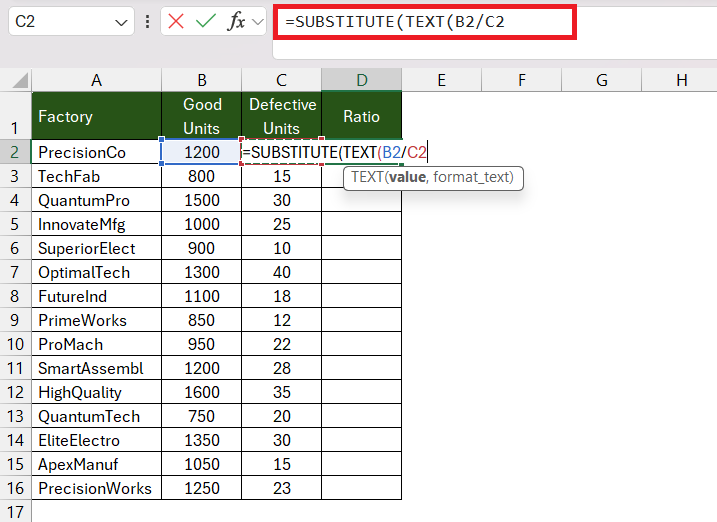
STEP 3: Enter the first argument of the text function i.e. division of the two numbers.
=SUBSTITUTE(TEXT(B2/C2
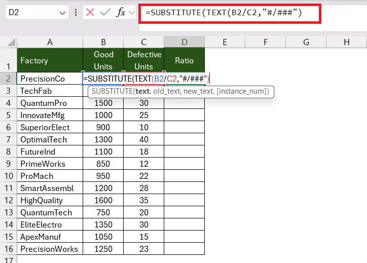
STEP 4: Enter the second argument of the text function i.e. “#/###”. This is the format to display the result as a fraction.
=SUBSTITUTE(TEXT(B2/C2,”#/###”)
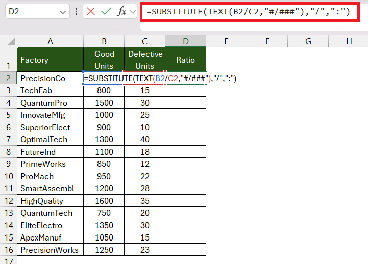
STEP 5: Enter the second argument of the substitute function i.e. the old text that you want to replace. Here, it is a forward slash (/).
=SUBSTITUTE(TEXT(B2/C2,”#/###”),”/”
STEP 6: Enter the third argument of the substitute function i.e. the new that will replace the old text. Here, it is a colon (:).
=SUBSTITUTE(TEXT(A2/B2,”#/###”),”/”,”:”)
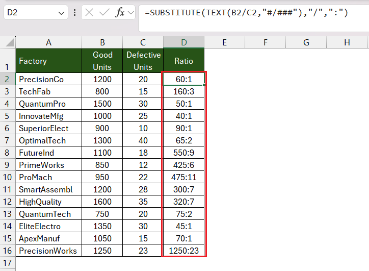
The ratio between goods produced and defective goods will be displayed in the format a:b.
Conclusion
In summary, this article explores four methods to calculate ratios in Microsoft Excel, catering to various scenarios and preferences.
The Simple Division method is easy but might not work well if the numbers don’t divide evenly. The GCD Function method leverages Excel’s GCD function to ensure accurate ratios. The Custom Format method is simple but can only show ratios with a slash (/). Lastly, the TEXT & SUBSTITUTE Function method provides a versatile approach to calculate and format ratios with a customizable separator, offering a balance between precision and presentation.
You can pick the method that fits your needs and the kind of data you have.
Learn more about Formulas with our 101 Advanced Excel Formulas & Functions Examples.
John Michaloudis is a former accountant and finance analyst at General Electric, a Microsoft MVP since 2020, an Amazon #1 bestselling author of 4 Microsoft Excel books and teacher of Microsoft Excel & Office over at his flagship Academy Online Course.
