Top 3 Methods to Locate Cell that Contains Specific Text in Excel

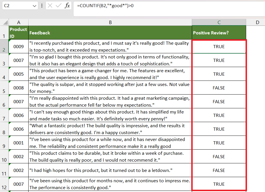
Although there isn’t a dedicated in-built Excel formula, there have 3 different ways that can be used to check what a cell contains  –

Let us delve into these functions thoroughly.

Download the Excel Workbook below to follow along and understand how to locate cell that contains specific text in Excel –

download excel workbookExcel-IF-Cell-Contains.xlsx

 

Using Find Feature

By following the steps provided below, it is possible to effectively locate positive feedback by utilizing a find feature in Excel.

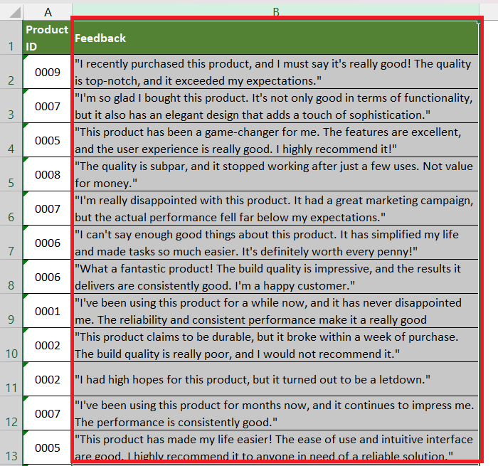
STEP 1: Select the range that contains all the feedback (i.e. Column B).

STEP 2: Go to Home > Find & Select > Find. Or, simply press Ctrl + F to open the Find dialog box.

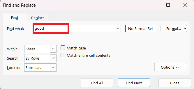
STEP 3: In the Find dialog box, enter the specific text you want to search. Here, it is the word “good”.

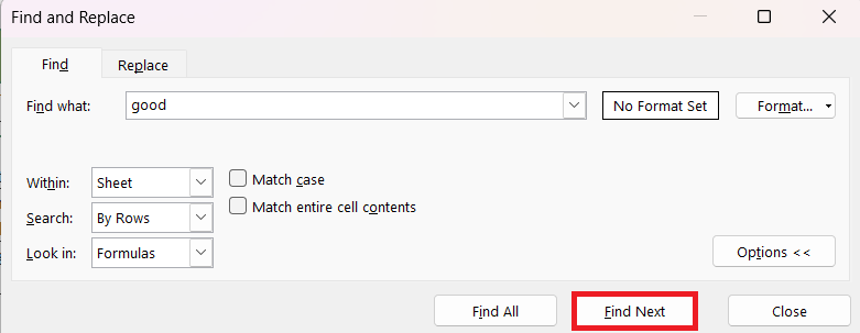
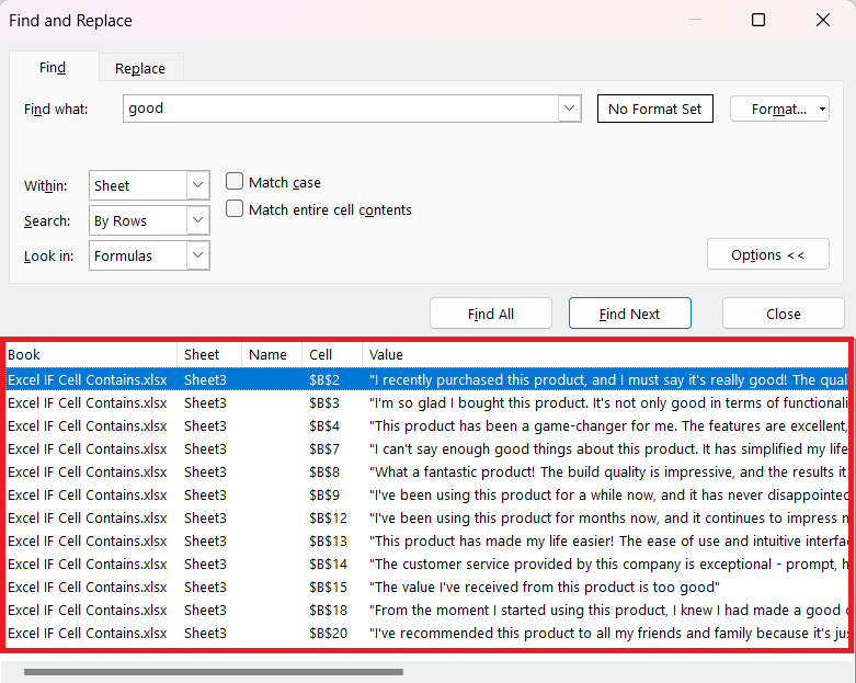
STEP 4: Click on the Find All button to display a list of all the cells containing the specified text.

All the cells that contain specific word i.e. good are displayed.

 

SEARCH Function

The SEARCH function is a text function in Excel used to get the starting position of a specified text in a text string. If the text is found, it returns the position or else it returns an error.

The syntax of the SEARCH function is –

=SEARCH(find_text, within_text, [start_num])

where,

• find_text: This is the text you want to find.
• within_text: This is the text string in which you want to search.
• start_num (optional): This specifies the character position from where the search should start.

You can combine SEARCH with ISNUMBER to get a boolean result i.e. TRUE and FALSE.

=ISNUMBER(SEARCH(find_text, within_text, [start_num]))

There can be 2 scenarios –

• Specified word is present – SEARCH will return the position and ISNUMBER will evaluate it as a number and return TRUE.
• Specified word is not present – SEARCH will return an error and ISNUMBER will return FALSE.

In this example, there are various products, and their feedback is mentioned in a table. You can easily find out the ones that are positive feedback (i.e. feedback contains the word “good”) using the SEARCH Function by following the steps below –

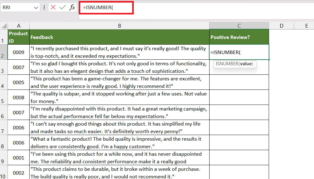
STEP 1: Enter the ISNUMBER function

=ISNUMBER(

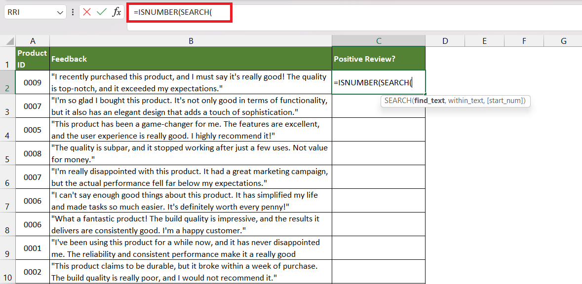
STEP 2: Enter the SEARCH function.

=ISNUMBER(SEARCH(

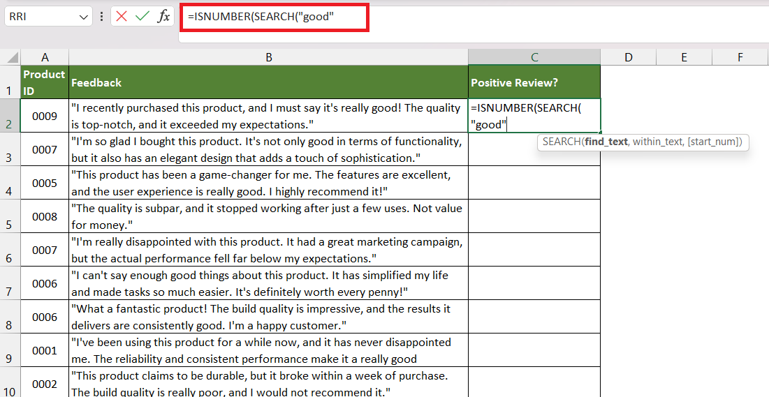
STEP 3: Enter the first argument of the search function i.e. find_text. Here, it is the word “good”.

=ISNUMBER(SEARCH(“good”,

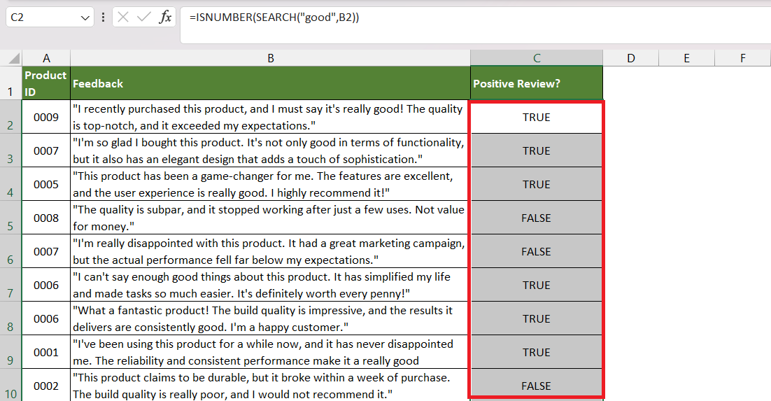
STEP 4: Enter the second argument of the search function i.e. within_text. Here, it is the cell B2.

=ISNUMBER(SEARCH(“good”,B2))

STEP 5: Copy the formula down.

 

COUNTIF Function

COUNTIF function is used to count the number of cells that match a specific condition. It can be employed to identify cells that contain the word “good”. Follow the steps below to understand how it can be done –

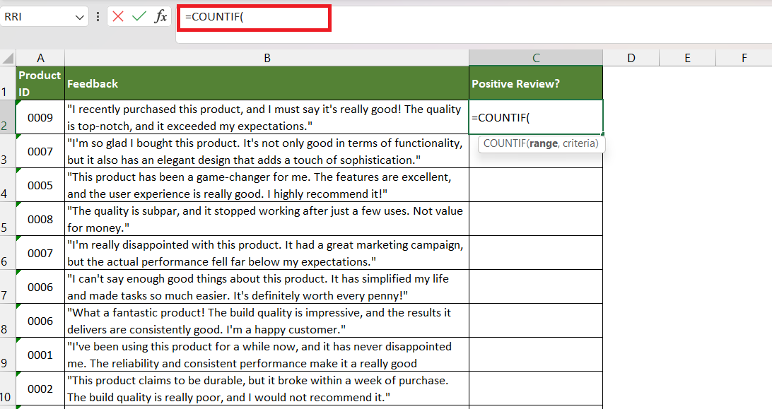
STEP 1: Enter the COUNTIF formula.

=COUNTIF(

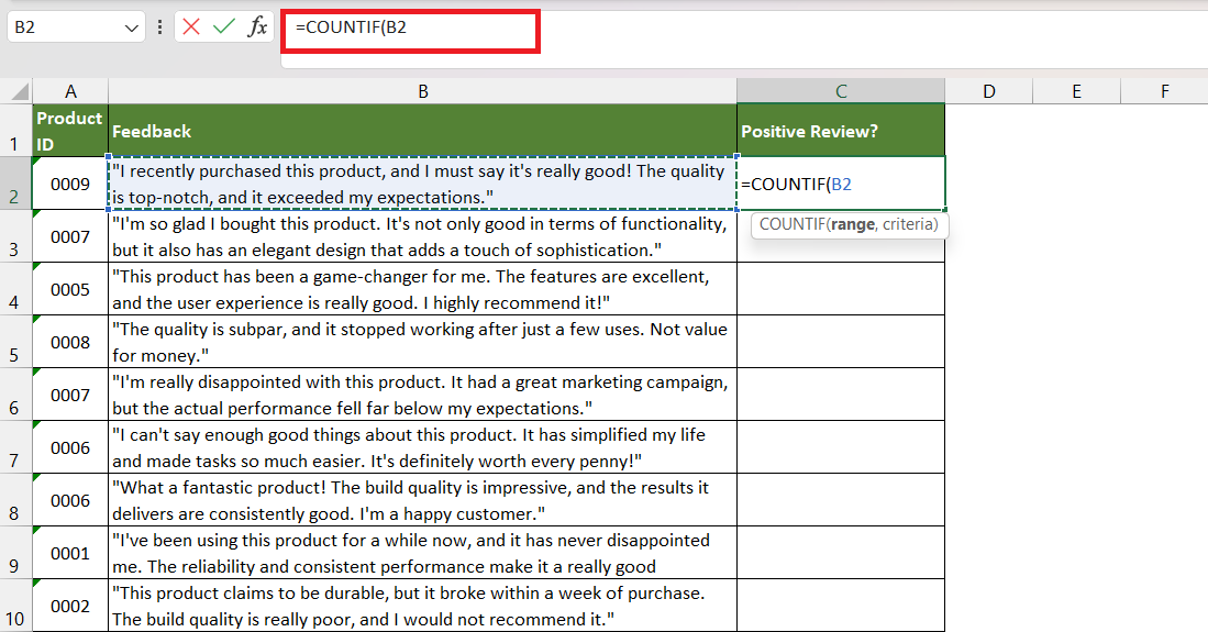
STEP 2: Enter the first argument i.e. the range of cells you want to search within. Here, it is the cell B2.

=COUNTIF(B2,

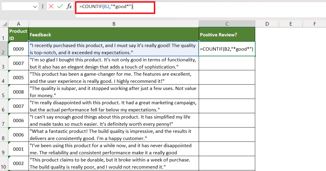
STEP 3: Enter the second argument i.e. criteria that you want to check against. Here, it is “*good*”.

=COUNTIF(B2,”*good*”)

The asterisks (*) act as wildcard characters, allowing for any text before and after the word “good”. This means that the formula will count cells that contain the word “good” anywhere within their contents, regardless of the surrounding text.

 

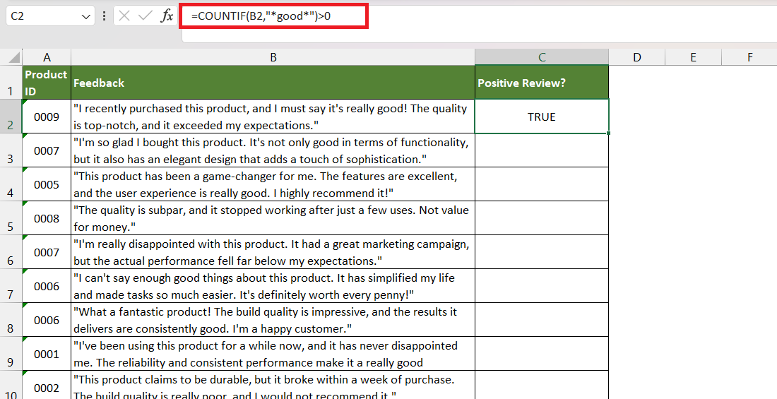
STEP 4: Enter the greater than operator followed by 0.

=COUNTIF(B2,”*good*”)>0

If the count is greater than zero, it means there is at least one occurrence of the word “good”. The function will return TRUE else FALSE.

 

STEP 5: Copy the formula down.

 

While Excel lacks a dedicated formula for identifying a cell that contains specific text, three methods are explored: utilizing the Find feature, combining the SEARCH function with ISNUMBER, and employing the COUNTIF function. Any one of these methods can be used to accomplish the desired result.