Change Count to Sum in Excel Pivot Tables

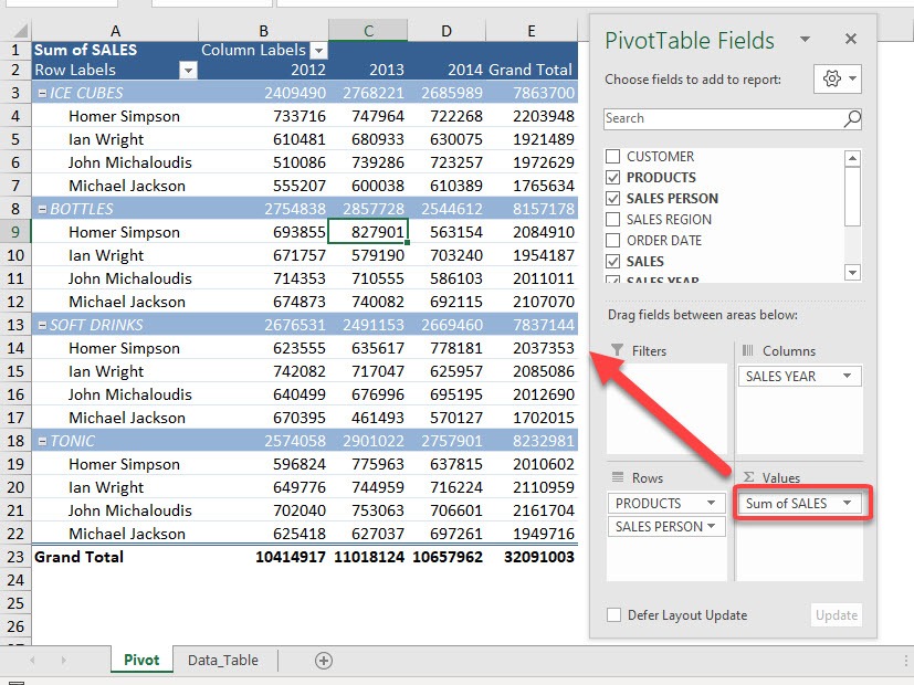
By default, when you put any field into the VALUES area of the pivot table it counts and displays the sum of the values. However, a much more common and needed function is the sum of the values of the field.

So let us see how we can change the COUNT to SUM in a Pivot Table.

Exercise Workbook:

Here is our Pivot Table, it’s currently set up to get the counts. But we want the sum of sales instead, so let us fix that pronto!

Method 1: Using the Pivot Table Fields tab.

STEP 1: Click on the arrow beside Count of SALES and select Value Field Settings

STEP 2: Select Sum and click OK

Now your Sales values are now being calculated as Sum instead of Count!

Method 2: Directly through the Pivot Table cells.

Additionally, you can also try this approach:

Step 1: Select any cell within the column.

Step 2: Right-click the cell and select Summarize Values By > Sum from the drop-down menu.

As you can see, the field value has now been updated to SUM instead of COUNT.

Make sure to download our FREE PDF on the 333 Excel keyboard Shortcuts here:

Bryan

Bryan is a best-selling book author of the 101 Excel Series paperback books.

See also  Sort an Excel Pivot Table Manually