Change Sum View in Label Areas

Exercise Workbook:

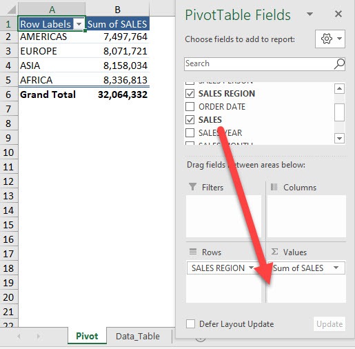
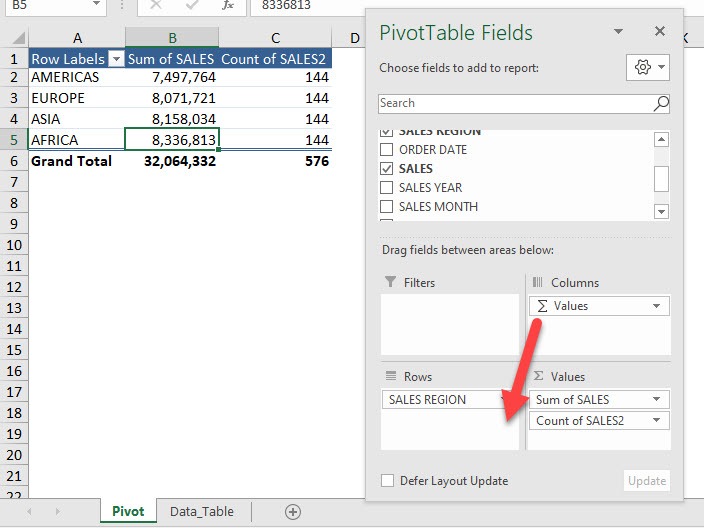
STEP 1: Here is our Pivot Table. Drag the Sales field to the Values area.

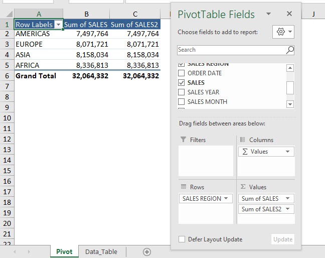
Notice we have the Sum of Values field added as well into the Columns area. This happens because we have more than one metric in our Values area.

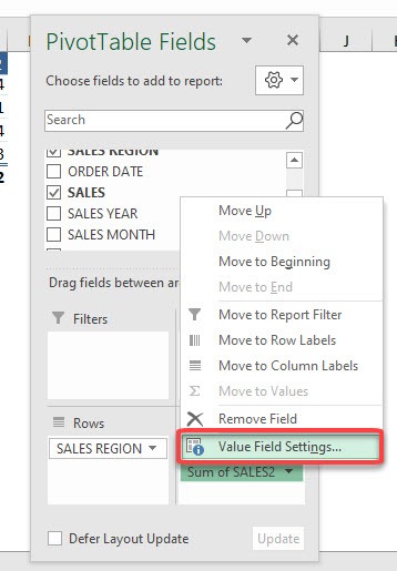
STEP 2: Let us change the second Sum of Sales field into Count. Click on the arrow and select Value Field Settings

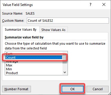
STEP 3: Select Count and click OK

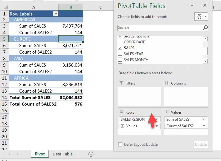
STEP 4: Now that we have our count, drag the Sum of Values field to the Rows area and see what happens!

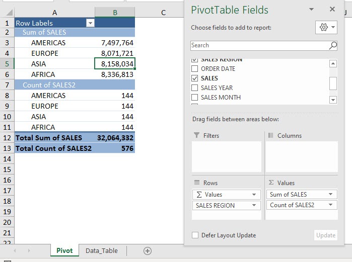
STEP 5: We have a completely different view. Now try moving the Sum of Values field above the SALES REGION field

And there you have the different views just by moving the Sum of Values field!

Make sure to download our FREE PDF on the 333 Excel keyboard Shortcuts here:

Bryan

Bryan is a best-selling book author of the 101 Excel Series paperback books.