The CHOOSE function in Microsoft Excel is a versatile tool designed to simplify data selection by returning a value from a specific position within a list. It introduces an efficient way to navigate through data based on set criteria, often enhancing productivity when combined with other Excel functions. Exploring the CHOOSE function’s capabilities can offer new dimensions in data manipulation and analysis, making it a valuable asset for any Excel user.
Key Takeaways
- The CHOOSE function in Excel simplifies data manipulation by allowing the selection of data based on specific criteria, enhancing workflow optimization.
- Analysts often utilize it for scenario analysis in financial models due to its simplicity and ease of comprehension when handling a modest number of scenarios.
- It is bound by a limitation of 254 arguments, setting a cap on the number of values or references that can be passed as inputs.
- While it is user-friendly for small-scale applications, it is less efficient than other Excel functions when dealing with larger, more complex datasets requiring extensive manual input.
Unveiling Excel’s CHOOSE Function
Understanding the Basics of CHOOSE
The CHOOSE function in Excel may seem like a hidden gem to many. At its core, the function allows you to select one of up to 254 values based on an index number. Think of it as a digital switchboard, guiding Excel to pick the exact information you need from a lineup of options.
The Syntax Behind the Power Tool
The syntax of the CHOOSE function is straightforward yet powerful. The function uses the following structure:
=CHOOSE(index_num, value1, [value2], ...).
Here, index_num specifies which value to return, where value1 is the first option, value2 the second, and so on. Excel will return the corresponding value that matches the number you indicate in index_num.
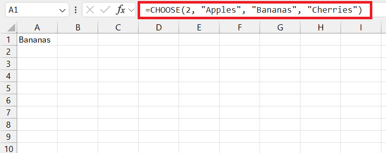
For example, CHOOSE(2, "Apples", "Bananas", "Cherries") would return “Bananas” because it is the second option listed.
Simplifying Data Sele with Quick Formulas Guide
Basic Examples That Illustrate Functionality
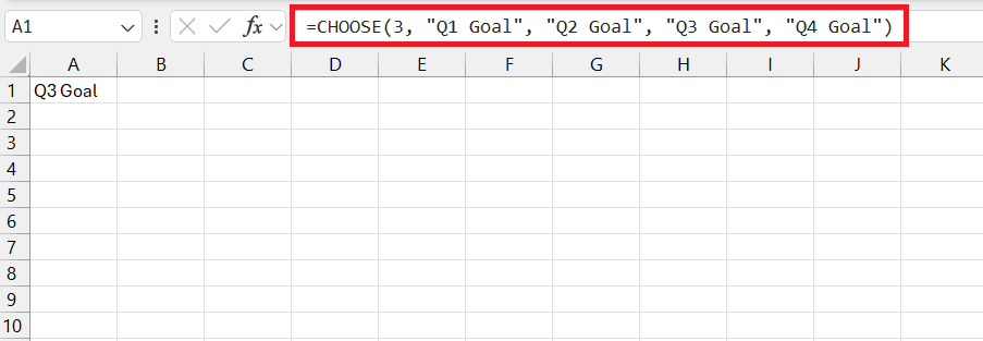
Diving into basic examples is a fantastic way to grasp how the CHOOSE function operates. Imagine you have a list of quarterly sales goals—Q1, Q2, Q3, and Q4—and you want to pick a specific goal:
=CHOOSE(3, "Q1 Goal", "Q2 Goal", "Q3 Goal", "Q4 Goal")
This formula would output “Q3 Goal” because you’ve set the index number to 3. Simple, right?
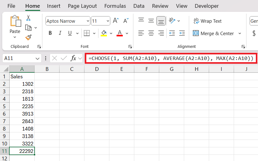
Another example could be switching between different data sets for analysis:
=CHOOSE(1, SUM(A2:A10), AVERAGE(A2:A10), MAX(A2:A10))
Here, by changing just the index number, you swiftly shift from summing to averaging or finding the max value within a range.
Advanced Scenarios for Real-world Application
Venturing into more complex territory, the CHOOSE function can be wielded to execute advanced scenarios that add sophistication to your data analysis. For instance, in financial modeling, you can utilize CHOOSE to navigate through different projections such as best, base, and worst-case scenarios:
=CHOOSE(scenario_number, "Base Case Revenue", "Best Case Revenue", "Worst Case Revenue")
In this formula, scenario_number is a cell reference where you set the scenario you want to analyze, and CHOOSE helps you toggle between the revenues for each case swiftly.
In project management dashboards, CHOOSE can dynamically select data based on the project phase:
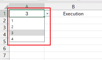
=CHOOSE(phase_number, "Initiation", "Planning", "Execution", "Closure")
By updating phase_number, the relevant phase information gets displayed without altering the entire dataset manually.
Beyond the Basics – Creative Uses of CHOOSE
Dynamic Dashboard Controls
Dynamic dashboards are the pinnacle of effective data presentation and the CHOOSE function plays a starring role in creating them. It can swiftly alter the data being displayed based on user interactions. For example, building a sales dashboard with CHOOSE allows you to switch between regions:
=CHOOSE(region_index, SUM(North_Sales), SUM(East_Sales), SUM(South_Sales), SUM(West_Sales))
Set up a control like a drop-down list linked to region_index, and your dashboard instantly updates to show the sales data for the selected region.
This interactive feature streamlines data analysis and enhances user experience, turning static spreadsheets into engaging reports.
Common Pitfalls and How to Avoid Them
Error Handling in CHOOSE Formulas
Error handling is crucial when working with CHOOSE formulas, as it can help prevent unexpected results and maintain data integrity. Here’s how you can manage potential errors:
#VALUE! Error: This occurs when index_num is out of range — either less than 1 or greater than the number of values provided in the function.
Use error-checking mechanisms such as IFERROR or conditional checks to handle this.
=IFERROR(CHOOSE(index_num, value1, value2), "Error message")
Data Validation: To avoid invalid index_num entries, employ data validation techniques by restricting the input to a certain range that corresponds to your values list.
Handling Non-Integer Indexes: Remember, if index_num is a fraction, CHOOSE truncates it to an integer. Use the INT function if there’s any risk of decimal values to ensure index integrity.
=CHOOSE(INT(index_num), value1, value2)
By anticipating and accounting for these errors, you ensure your CHOOSE function operates seamlessly within your Excel models.
Performance Tips for Large Datasets
When dealing with large datasets, maintaining performance is key. Here are some tips to optimize the performance of the CHOOSE function:
Streamline Data Ranges: Tighten the focus of your referenced ranges. Avoid referencing entire columns if you only need a small data subset — this saves memory and processing power.
Avoid Volatile Functions: Refrain from coupling CHOOSE with volatile functions like TODAY or INDIRECT, especially in large worksheets, as they can trigger unnecessary recalculations.
Calculation Settings: For datasets that require heavy computation, consider switching Excel to manual calculation mode while building your model. This way, Excel will only recalculate when you tell it to.
Use Helper Columns: Break complex operations into steps and use helper columns instead of nesting many functions within CHOOSE. This makes the workbook easier to debug and can improve performance.
Compress Data When Possible: Consider employing data compression techniques such as removing duplicates and outliers or using data summarization before feeding it into the CHOOSE function.
Incorporating these performance tips ensures that even with extensive use of the CHOOSE function, your Excel workbooks remain responsive and efficient.
Integrating CHOOSE with Other Excel Functions
Coupling CHOOSE with Lookup Functions
Integrating the CHOOSE function with lookup functions can unlock even greater flexibility in your Excel tasks. Here’s how they complement each other:
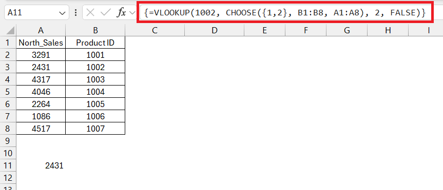
Rewiring VLOOKUP for Leftward Searches: VLOOKUP traditionally searches to the right, but with CHOOSE, you can restructure your range to pull data from the left:
=VLOOKUP(value, CHOOSE({1,2}, lookup_range_column_to_return, lookup_range_column_to_search), 2, FALSE)
This way, the search column becomes the second column in the virtual array created by CHOOSE, circumventing VLOOKUP’s limitation.
Enhancing HLOOKUP with Dynamic Headers: Similarly, you can use CHOOSE to dynamically define the row headers for HLOOKUP, allowing flexible row-based searching.
=HLOOKUP(value, CHOOSE({1,2}, header1, header2, header3), row_index, FALSE)
Combining with another CHOOSE: While CHOOSE is powerful on its own, its versatility is further extended when used in conjunction with itself, creating nested CHOOSE functions. This technique allows for more complex decision-making processes.
=CHOOSE(1,CHOOSE(3,2000,2001,2002),2003,2004,2005)
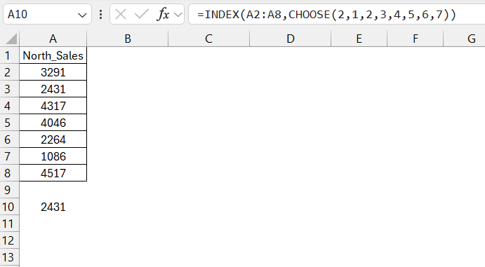
Combine with INDEX: You can use CHOOSE in conjunction with the INDEX function to create more advanced lookup scenarios. Cell A1 contains an index, the CHOOSE function determines which element of the array to select using the INDEX function.
=INDEX(array,CHOOSE(index_num,value1,value2,...))
Harnessing the synergy between these functions allows for sophisticated data retrieval and expands the versatility of search tasks in Excel.
Frequently Asked Questions
What are the limits of the CHOOSE function in Excel?
The major limit of the CHOOSE function in Excel is that it can handle only up to 254 values or references as arguments. Any index number outside the range of 1 to 254 will result in an error, and using more than 254 values will not be possible.
Can CHOOSE Function replace nested IFs effectively?
Yes, the CHOOSE function can efficiently replace nested IF statements in many cases, especially when dealing with a predefined set of conditions. It simplifies formulas by mapping index numbers to specific outcomes, avoiding the complexity of multiple IF layers.
What function can automatically return the value in cell?
The CHOOSE function is typically used for selecting a value from a list based on a specified index or position. It allows you to create a list of values and select one of them by specifying the position number.
What is the difference between VLOOKUP and CHOOSE?
VLOOKUP is designed to search for a value in the first column of a table and return a value in the same row from a specified column. CHOOSE, on the other hand, lets you select a value or action based on its position in a list you provide. While VLOOKUP is for vertical lookup in ranges, CHOOSE is for selecting among several provided options.
John Michaloudis is a former accountant and finance analyst at General Electric, a Microsoft MVP since 2020, an Amazon #1 bestselling author of 4 Microsoft Excel books and teacher of Microsoft Excel & Office over at his flagship Academy Online Course.
