Clean Data Set for Pivot Table

• When your data is not clean
• How to clean your data.

Exercise Workbook:

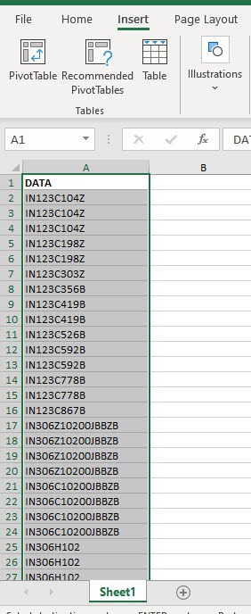
STEP 1: Here is our data set, select the data and go to Insert > Tables > PivotTable

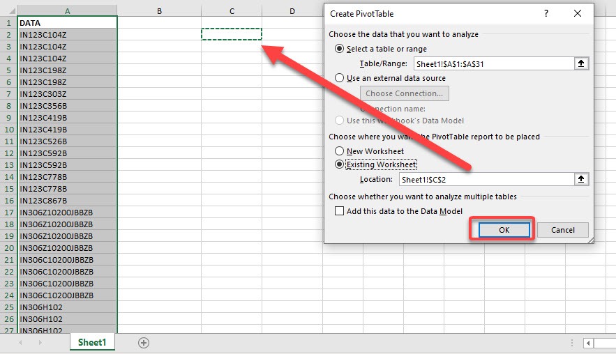
STEP 2: Select Existing Worksheet and pick a cell inside the same worksheet to insert our Pivot Table. Click OK.

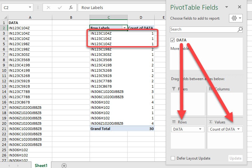
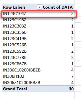
STEP 3: Drag the DATA column into Rows and Values

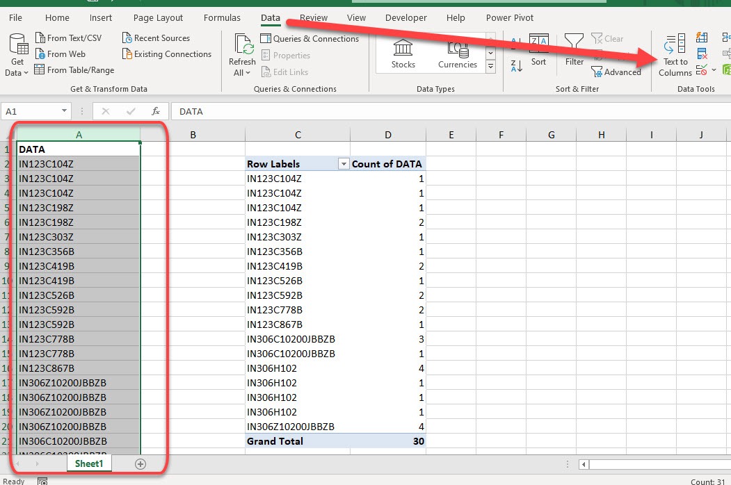
You will notice that how come IN123C104Z is appearing as 3 rows? This is caused by our dirty data!

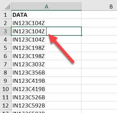
STEP 4: If you inspect the data table closely, you will see that they have extra spaces. This is what’s causing our Pivot Table to have weird outputs!

STEP 5: Let us clean those extra spaces! Select the entire column of your data and go to Data > Data Tools > Text to Columns

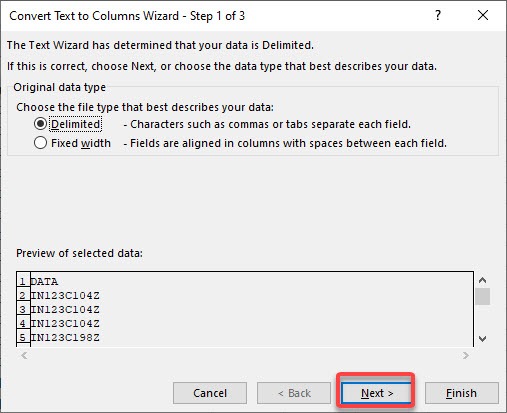
STEP 6: Click Next

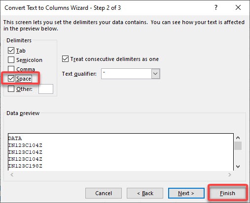
STEP 7: Make sure Space is ticked and select Finish. This will remove the extra spaces as a result.

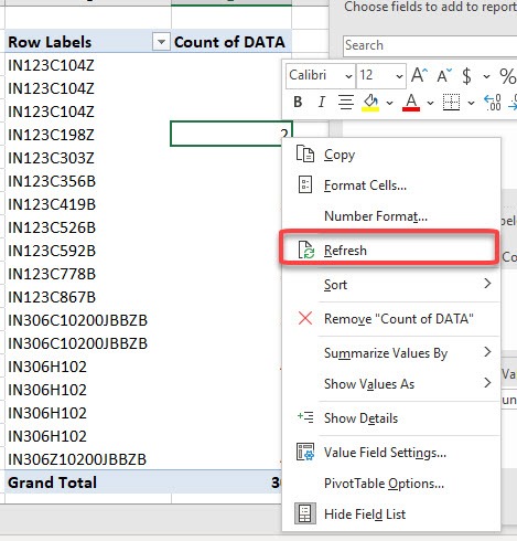
STEP 8: Right click anywhere on your Pivot Table and select Refresh to reflect our data cleanup.

Now that’s looking much better!

Bryan

Bryan is a best-selling book author of the 101 Excel Series paperback books.