Many times, you may have faced the problem that Excel is not returning the desired value, instead is showing an error. The most common one amongst these is a#REF! error in Excel.
A #REF error in Excel is shown when the cell reference provided in a formula is not valid. It is important to know why this error occurs and how to fix it.
In this article, you will learn the following:
What is #REF! error in Excel?
What does #REF mean in Excel? #REF! error stands of reference i.e. this error is shown when the cell that is referenced to in a formula is no longer valid or does not exist.
So, #REF error in Excel occurs when the reference used is invalid. It can happen due to one of the following reasons:
- Row, column or sheet has been deleted.
- Formula contains incorrect or invalid cell reference.
This means that Excel returns a #REF error when the formula refers to a cell that isn’t valid.
Let’s look at a few examples to see when this error occurs and how to fix it!
How to fix #REF error in Excel?
Example 1:
Watch the YouTube video to learn how to fix #REF error in Excel and if you like it give it a thumbs-up!
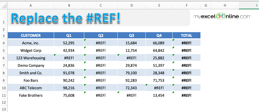
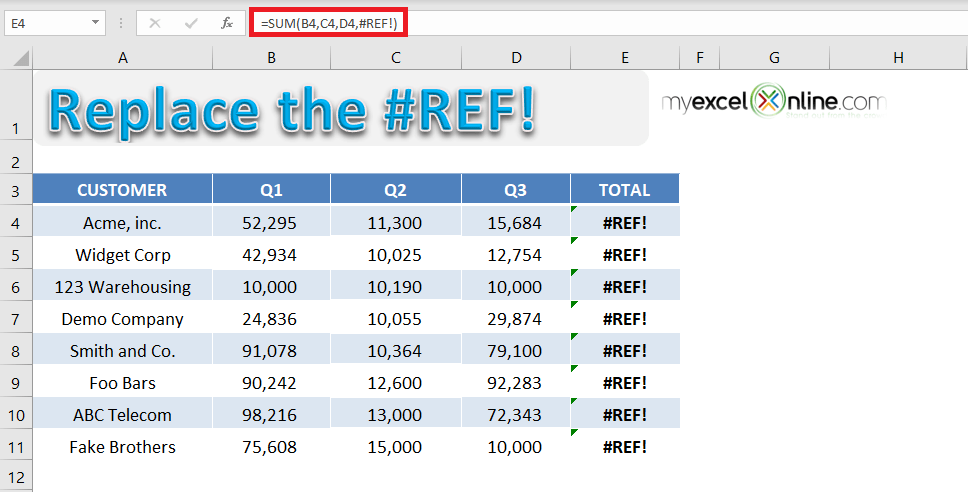
In the table below, you will spot multiple #REF! error within formulas used in the cell.
This has happened because you have deleted a range that contains an explicit cell reference within the formula used.
To get rid of this error message we have to select the cell(s) with this error, use the Find & Replace dialog box and do the following:
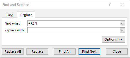
Find What: #REF!
Replace With: (Leave this blank)
Press OK and it will clear the #REF error in Excel within the formula.
Let’s look at the step-by-step tutorial below to understand how to remove #REF in Excel.
Download the workbook and follow along:
Download workbookReplace-the-REF-error-2.xlsx
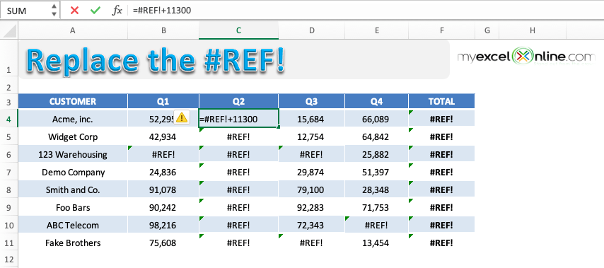
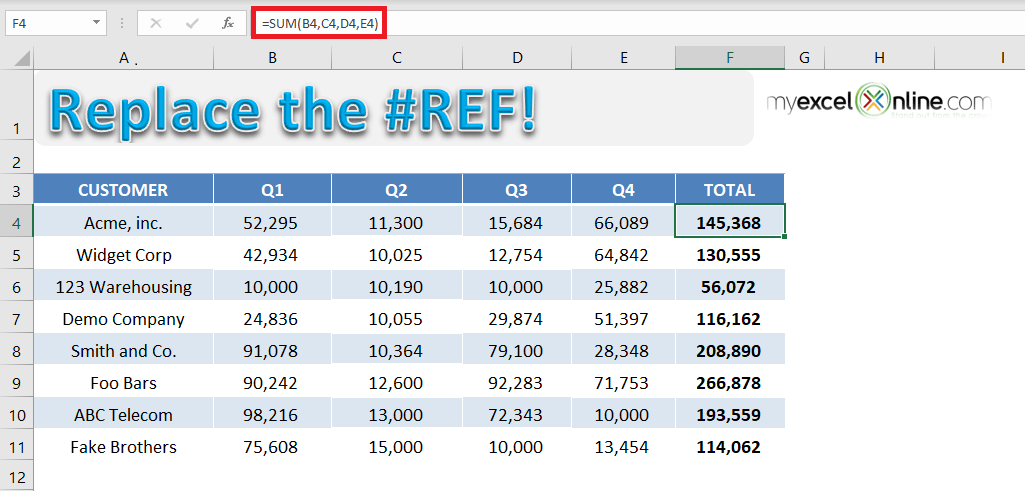
STEP 1: To check the cell containing the cell, simply click on the cell and press F2.
Here, since you have used an explicit cell reference and it was deleted, Excel is returning a #REF error.
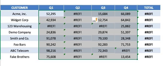
STEP 2: Highlight the table containing the errors.
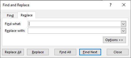
STEP 3: Press Ctrl + H to open the Find & Replace dialog box.
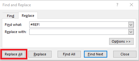
STEP 4: Under Find What, input #REF! and leave Replace as blank. This is done to replace all the #REF! error with a blank.
STEP 5: Click on Replace All.
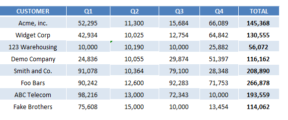
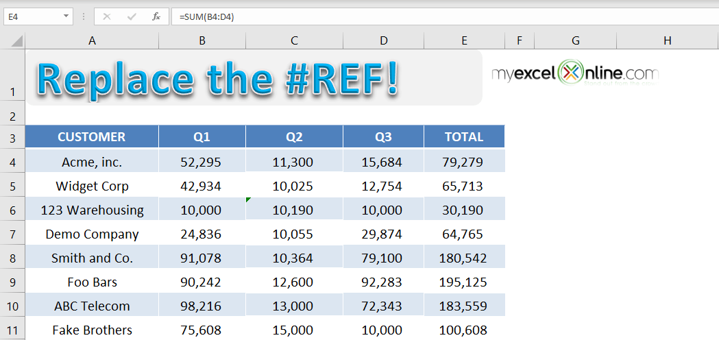
This is how your replaced data will look like:
Let’s look at another example when this error occurs due to copy-pasting the formula from other cells.
Example 2:
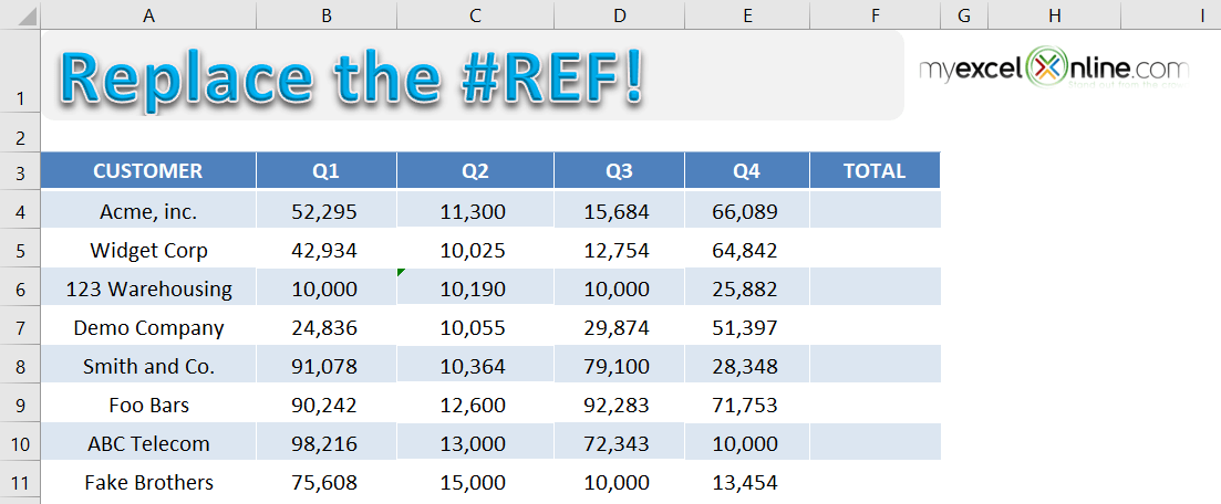
In the table below, you have sales data for different customers for 4 quarters and a sum formula used to calculate the total sales. The formula used to calculate the total sales value is =SUM(B4, C4, D4, E4).
If you try and delete Column E (Quarter 4), the sum formula will change to =SUM(B4, C4, D4,#REF!) and return an error – #REF.
This error is caused because the formula to calculate the total sales uses explicit cell reference. When one of the cell references used in the formula is deleted (here cell E4), Excel is unable to calculate the value and returns an error.
A simple fix to this problem is to use a range instead of an explicit cell reference. Let’s look at the step-by-step tutorial to learn how:
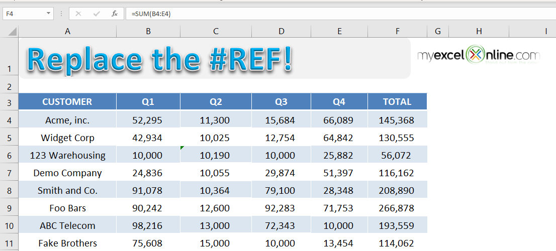
STEP 1: Use formula =SUM(B4: E4) in cell F4 and copy-paste the formula below to cells F5: F11.
STEP 2: Now delete the Column E to get the total sales for only 3 quarters.
If you change the formula from =SUM(B4, C4, D4, E4) to =SUM(B4: E4), you will no longer to vulnerable to #REF in Excel. This formula recalculates the total sales value by removing the deleted cell.
Hence, it is advised to use range while writing a formula instead of explicit cell reference.
Let’s take a look at another example when the error occurred due to VLOOKUP containing invalid cell reference.
Example 3:
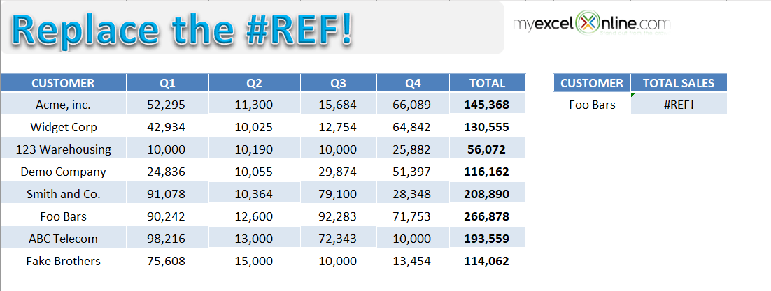
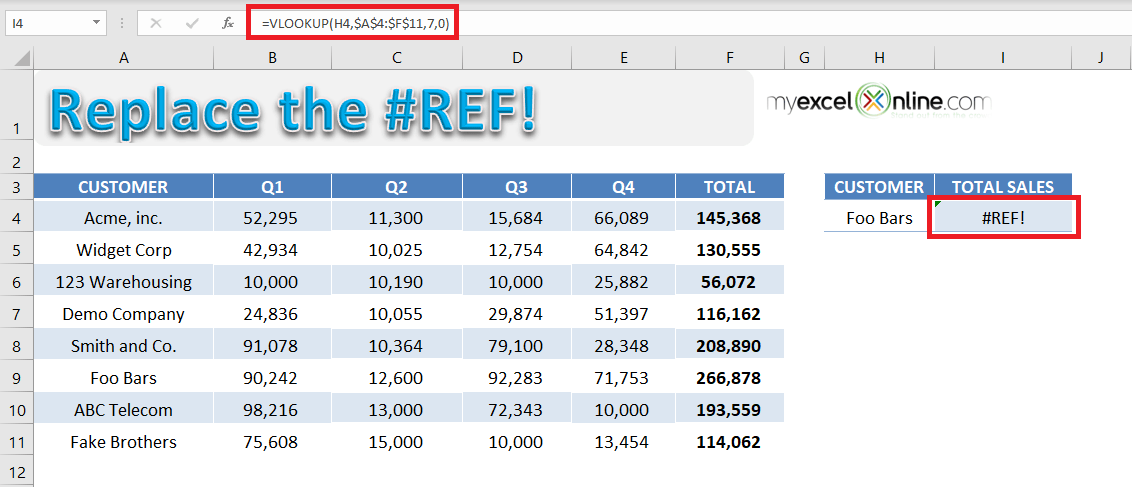
In the table below you have quarterly and total sales for different customers and using the VLOOKUP formula, you have tried to find out the total sales for the customer name mentioned.
The formula used to find the total sales for customers mentioned in cell H4 is =VLOOKUP(H4,$A$4:$F$11,7,0).
If you look into the formula used in detail, you will see that the value used to indicate the column index number is incorrect.
The arguments for a VLOOKUP function is:
- Lookup_value = The value you want to look up in the first column of the table.
- Table_array = The table from which you need to retrieve the data.
- Col_index_num = The column number in the table array from which matching value should be returned.
- Range_lookup = Value should be 1 if you want an approximate match or 0 if you want an exact match of the return value.
Excel is returning an error in this formula because VLOOKUP is looking to return a value from the 7th column but the reference $A$4:$F$11 contains only 6 columns.
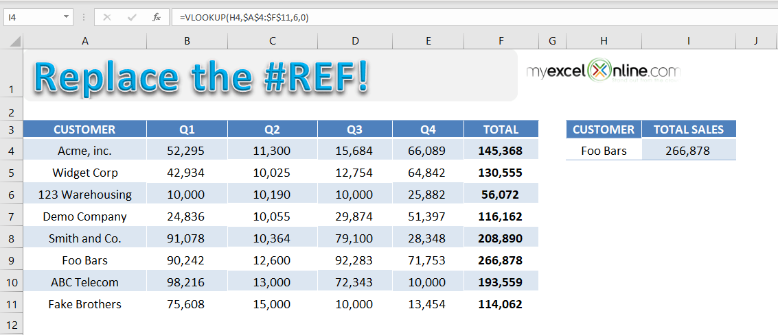
To fix this error, use the formula =VLOOKUP(H4,$A$4:$F$11,6,0).
Conclusion
Excel returns #REF error to indicate that the cell reference used in the formula is not valid. It may be because the referred cell, row, or column has been deleted or the range used in the formula is incorrect.
With the help of this tutorial, you will be able to spot a #REF error in Excel and learn how to fix #REF in Excel.
HELPFUL RESOURCE:
To learn how to correct the Hash Error, click here.
Make sure to download our FREE PDF on the 333 Excel keyboard Shortcuts here:
You can learn more about how to use Excel by viewing our FREE Excel webinar training on Formulas, Pivot Tables, and Macros & VBA!
John Michaloudis is a former accountant and finance analyst at General Electric, a Microsoft MVP since 2020, an Amazon #1 bestselling author of 4 Microsoft Excel books and teacher of Microsoft Excel & Office over at his flagship Academy Online Course.

