How to Use Conditional Formatting Based on Another Cell

Say you want a cell to be highlighted once its’ values hit a certain threshold. If you can format the appearance of cells, your data will be easier to understand. You will also be able to focus on the formatted cells leading to streamlined decision-making. In this article, we will explore the steps on how to use conditional formatting based on another cell.

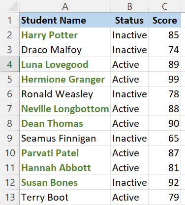
Our final product will look like this:

In this example, we want to highlight the name of the students in column A who have a mark above 80 on column C, indicating their passing status.

Let’s go through these steps thoroughly!

Download the Excel Workbook below to follow along How to Use Conditional Formatting Based on Another Cell! –

download excel workbook ConditionalFormattingBasedonAnotherCell.xlsx

Based on One Cell

The first step is to create your new conditional formatting rule.

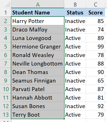
Highlight the range of names from A2 to A13.

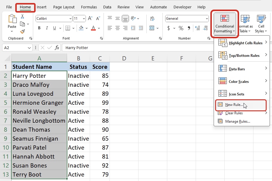
Go to the Home tab and click on Conditional Formatting.

Select New Rule.

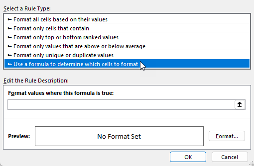
Click on Use a formula to determine which cells to format.

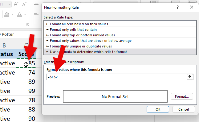
Under the Format values where this formula is true, type in the = sign and click on C2.

As you can see, Excel will automatically consider cell C2 as an absolute reference as it put the $ sign in front of both column C and row 2. To allow this formula to copy down to the other rows, it is important for us to delete the $ sign in front of row 2 to make it a relative reference.

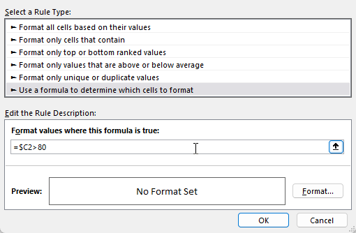
Type in the final formula as =$C2>80.

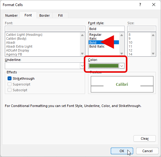
Click on Format to decide on how you want the names that meet the condition to look. You can modify the cells based on font color, background color, borders, and other formatting choices. In our example, we will select bold and the color green. Click OK.

As you can see, the names of the students in column A are highlighted based on their passing score on column C.

Bonus: Formatting Based on Multiple Cells

What if we wanted to highlight cells based on multiple conditions from multiple cells?

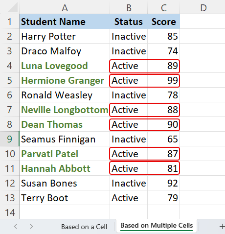
Let’s say we only want to highlight the student names in Column A if their status in Column B is Active AND their score in Column C is higher than 80.

Select the range.

Go to the Home tab and click on Conditional Formatting.

Select New Rule.

Click on Use a formula to determine which cells to format.

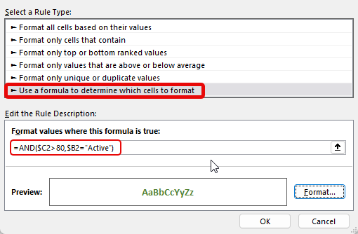
Enter the formula =AND($C2>80, $B2=“Active”). This formula is basically saying we want to format values where this formula is true if the cell in column C is greater than 80 AND if the cell in column B is active.

Choose the Format you would like the cells to be in and click OK.

As you can see, only the names of the students in column A are highlighted based on their passing score above 80 in column C and their active status in column B.

Conclusion:
There you have it! Conditional formatting based on another cell is one of the most useful ways to bring clarity to your data. It works perfectly well with formulas, as well. Make sure you use these skills the next time you work on a spreadsheet!