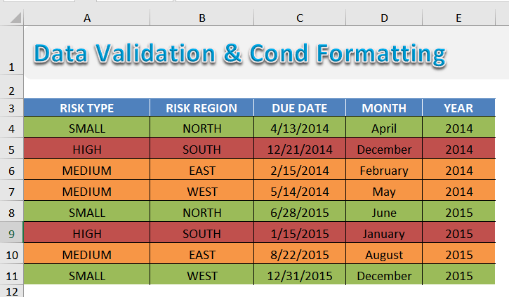
In a previous post I showed you how to Create a Drop Down List in a Table. We are now going to take this concept one level further and apply some conditional formatting to the drop down data validation list.
This is useful if you want to highlight when a job is completed, check off items from a list or to evaluate risk in a project just like I have done in below´s example.
Table of Contents
Want to know all about Conditional Formatting from Beginner to Advanced?
*** Watch our video and step by step guide below with free downloadable Excel workbook to practice ***
Watch it on YouTube and give it a thumbs-up!
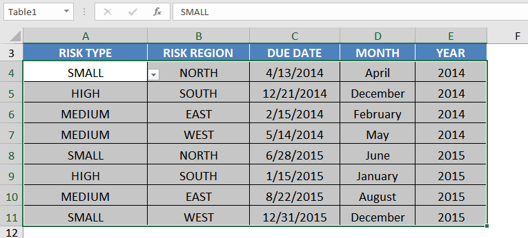
STEP 1: Select the range that you want to apply the conditional formatting to.
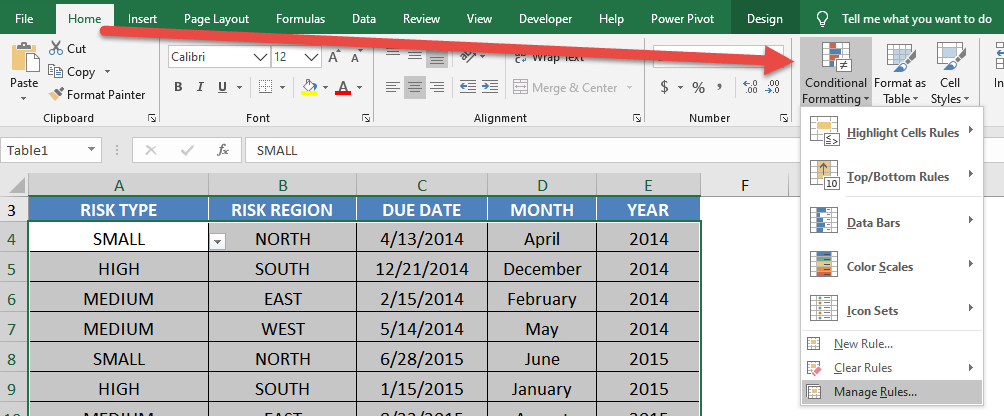
STEP 2: Go to Home > Styles > Conditional Formatting > Manage Rules
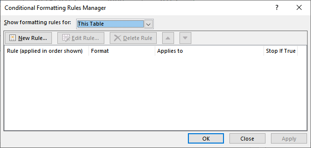
STEP 3: Select New Rule
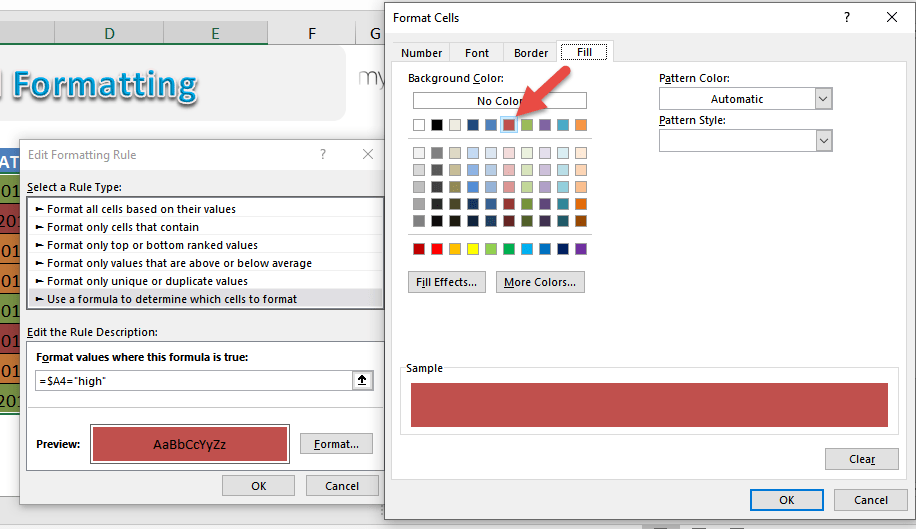
STEP 4: Create the new rule for High values:
Select Use a formula to determine which cells to format
Type in the Formula =$A4=”high”
This formula will ensure only the column is absolute.
Go to Format > Fill then select a color of your choosing. Click OK.
Repeat the same steps for medium values. Click New Rule.
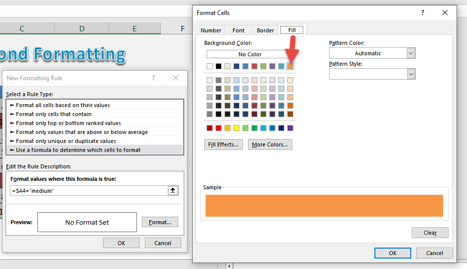
Select Use a formula to determine which cells to format
Type in the Formula =$A4=”medium”
This formula will ensure only the column is absolute.
Go to Format > Fill then select a color of your choosing. Click OK.
Repeat the same steps for low values. Click New Rule.
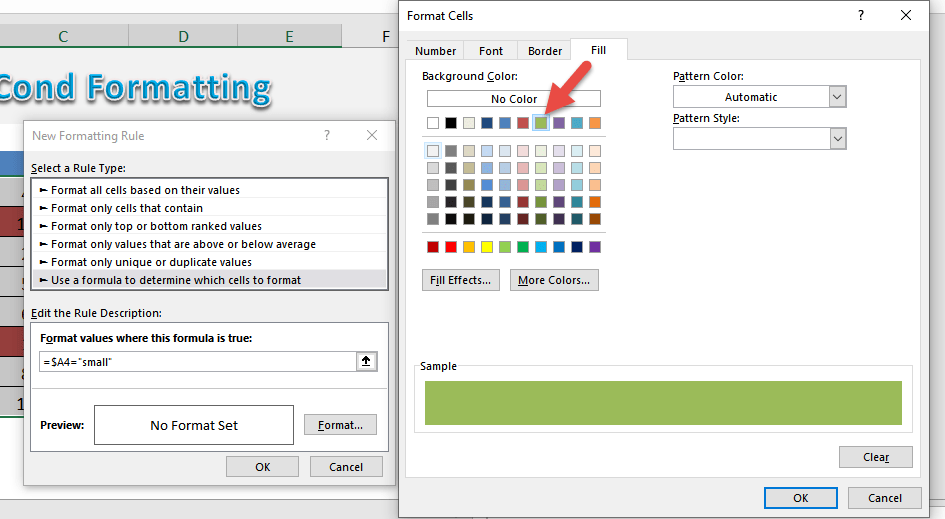
Select Use a formula to determine which cells to format
Type in the Formula =$A4=”low”
This formula will ensure only the column is absolute.
Go to Format > Fill then select a color of your choosing. Click OK.
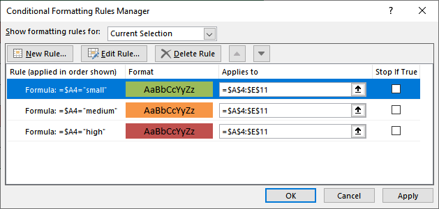
This is how our new set of rules will look like:
Now our table now has conditional formatting applied!
Further Learning:
- Conditionally Format a Pivot Table With Data Bars
- Select & Format Fields in Excel Pivot Tables
- Replace Excel Formatting with Another Formatting
Helpful Resource:
To learn how to add a drop down menu in your Excel Table, click here.
John Michaloudis is a former accountant and finance analyst at General Electric, a Microsoft MVP since 2020, an Amazon #1 bestselling author of 4 Microsoft Excel books and teacher of Microsoft Excel & Office over at his flagship Academy Online Course.
