The article dives into the essentials of the COUNTIF function in Microsoft Excel, revealing its potential for simple to complex data analysis tasks. From its basic single-criterion usage to advanced applications with multiple conditions, the piece offers a comprehensive guide to mastering this versatile tool. Through practical examples and insightful tips, readers learn to navigate COUNTIF’s capabilities and limitations, enhancing their analytical skills in Excel.
Key Takeaways
- Understanding the basic syntax of COUNTIF (=COUNTIF(range, criteria)) is crucial for effectively utilizing Excel for data analysis, allowing for the counting of cells based on various data types and conditions.
- The COUNTIF function in Excel is used to count the number of cells that meet a single condition within a range.
- For more complex analyses requiring multiple criteria, COUNTIFS or a combination of COUNTIF with other functions can refine queries and extract precise information, significantly expanding the function’s utility.
- While single-criteria COUNTIF is straightforward and suitable for simple queries, mastering multiple criteria with COUNTIFS is essential for nuanced, multi-dimensional data analysis.
- Practical examples, such as using COUNTIF with AND/OR logic and leveraging wildcards for flexible criteria matching, illustrate the function’s adaptability to real-world data challenges.
Download the practice worksheet and follow the blog on How to Master COUNTIF with Multiple Criteria in Excel – Download excel workbookCOUNTIF-Multiple-Criteria-in-Excel.xlsx
Table of Contents
Unlocking the Power of Excel COUNTIF with Multiple Criteria
Understanding COUNTIF’s Basic Functionality
Excel’s COUNTIF function is pivotal for users who need to count cells that match a specific criterion. At its most fundamental, COUNTIF combines two essential elements: a range of cells to examine and the criteria for which to count the cells.
For ease, think of COUNTIF’s basic syntax like this: =COUNTIF(range, criteria). This formula structure can handle various data types including numbers, dates, texts, or even expressions like “>32. By mastering this function, you start unlocking Excel’s potential for efficient data analysis.
Diving into Complex Data Analysis with Multiple Criteria
When your data analysis requires more sophistication than a simple count, deploying COUNTIF with multiple criteria argument becomes invaluable. This usually means you’re looking to count cells that match various conditions simultaneously, which calls for an understanding of how to extend the basic COUNTIF functionality.
For example, you might be monitoring financials and want to count how many companies have a market capitalization above a certain threshold, but also exhibit a price-to-earnings ratio within a particular range.
Unfortunately, COUNTIF alone isn’t equipped for such intricacies, but by using COUNTIFS, an extension of COUNTIF, or combining it with other functions, you can set up multiple criteria effectively. This advanced utility helps you refine your queries and extract more precise information from your datasets.
Mastering Single vs. Multiple Criteria in COUNTIF
The Simplified World of Single-Criteria COUNTIF
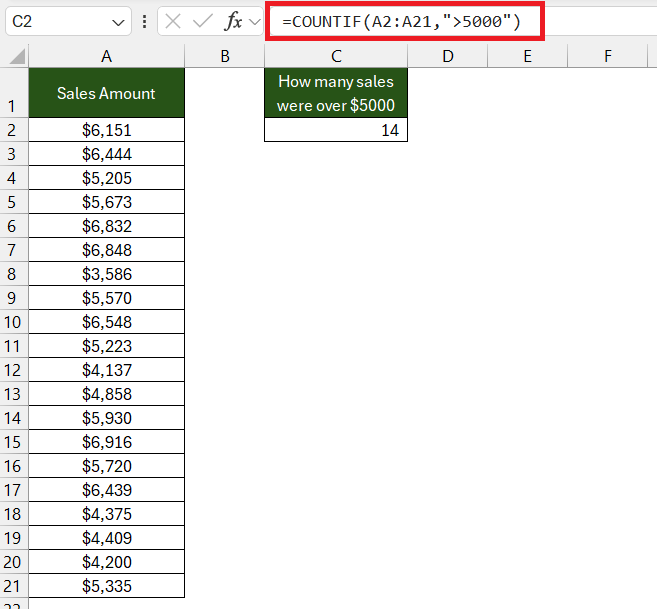
For those who are new to Excel or prefer straightforward data tasks, the single-criteria COUNTIF is a go-to tool. Its simplicity lies in its ability to focus on one condition at a time, such as counting how many times a certain value appears within a range. Think of it as asking a single, direct question of your data: “How many sales were over $5000?” or “How many tasks are marked as ‘Complete’?”
The COUNTIF function returns the number of cells that match the specified criterion, and with its simplicity and ease, it’s a quick way to gain insights without wading through complexities. Remember, the basic form looks like this: =COUNTIF(range, "criteria"). This singular focus can serve as an excellent starting point for more involved data analysis.
Navigating Through Advanced Scenarios Using Multiple Criteria
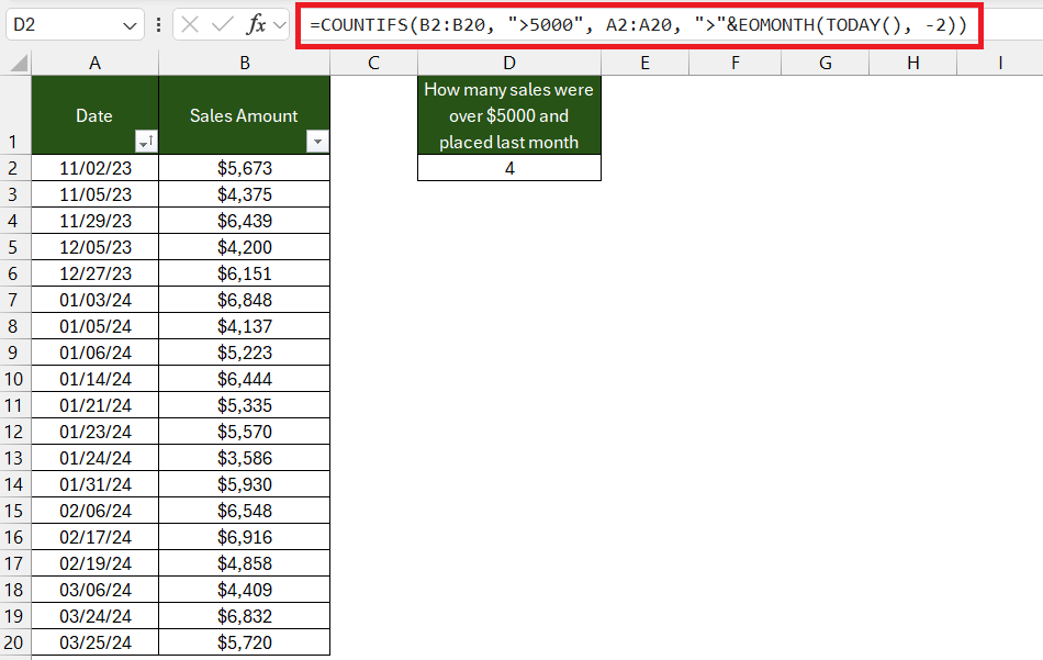
As you delve deeper into data, situations often demand more nuanced analysis – this is where multiple criteria become essential. For instance, you might need to know how many products fall into a high-profit, high-demand category, requiring counts based on multiple conditions. To navigate these advanced scenarios, you’ll use the COUNTIFS function, which can handle several conditions across different ranges.
Let’s consider a practical example: you want to count the number of orders that are above $5000 and were placed in the past 2 months. With COUNTIFS, your formula would look something like this: =COUNTIFS(PriceRange, ">5000", DateRange, ">"&EOMONTH(TODAY(), -2)).
Here, you’re pairing each range with its respective criterion, allowing COUNTIF to perform multidimensional analysis.
While COUNTIFS opens up a world of possibilities, there are tricks to getting it just right – like ensuring your ranges are the same size and understanding how to align each criterion with its related range. When mastered, this capability becomes a powerful part of your Excel skillset, enabling sophisticated assessments of your data.
Real-World Examples to Illustrate COUNTIF Flexibility
Case Study: COUNTIF with AND Logic
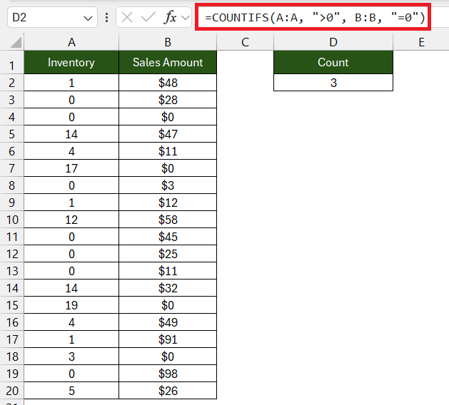
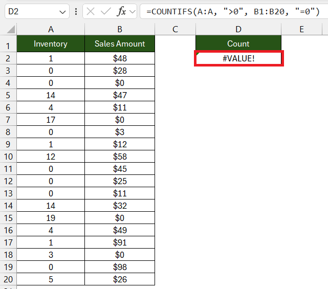
Using COUNTIF with AND logic seems straightforward since COUNTIFS inherently applies AND logic to its multiple criteria. Let’s illustrate this with a practical example: you’re managing an inventory and want to identify items that are in stock but haven’t been sold yet. This requires counting cells based on two criteria—the stock counts have to be greater than zero, and the sold counts need to be zero.
You would use the following COUNTIFS formula to achieve this: =COUNTIFS(A:A, ">0", B:B, "=0"). This formula counts only the rows where there’s available stock (Column A greater than 0) and no sales (Column B equal to 0).
The result reveals the number of items meeting both conditions simultaneously.
Such scenarios present a common use case in inventory management, data analysis, and reporting where a dual criterion count can provide critical insights into a dataset’s status or performance.
Case Study: COUNTIF with OR Logic
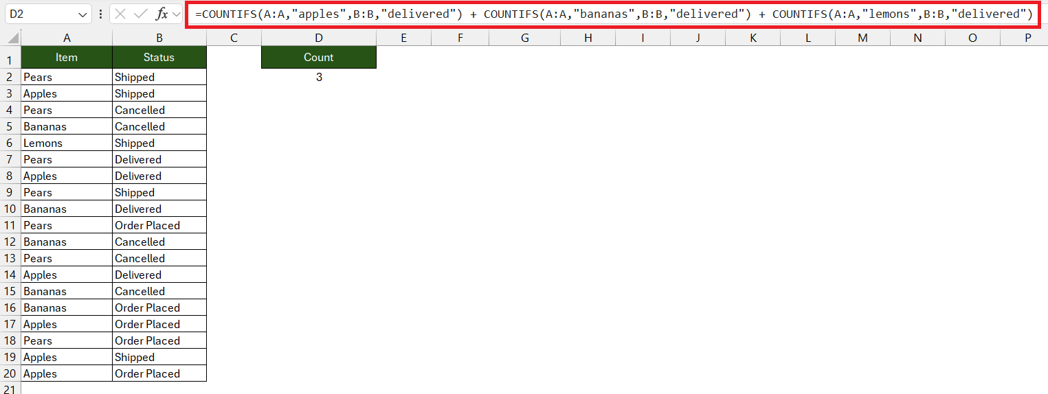
Counting cells that satisfy one or more conditions from a set can be tricky, as Excel’s COUNTIFS function defaults to an AND logic, meaning all criteria must be met simultaneously. So, how do you count using OR logic? Imagine you need to tally “apples”, “bananas”, or “lemons” that are labeled as “delivered”. In Excel’s language, your criteria would be set as:
- For Column A: “apples” OR “bananas” OR “lemons”
- For Column C: “delivered”
To achieve this count, you’ll need to craft a formula that handles the OR conditions. A typical solution involves summing separate COUNTIFS for each condition. Here’s how it’s done: =COUNTIFS(A:A,"apples",B:B,"delivered") + COUNTIFS(A:A,"bananas",B:B,"delivered") + COUNTIFS(A:A,"lemons",B:B,"delivered"). You’re separately counting for each fruit that’s delivered and summing the counts to get the total.
This example demonstrates the flexibility of COUNTIF and COUNTIFS, showing they can be creatively combined to suit your data needs, even when the default function behavior doesn’t match your logic requirements.
Pushing Boundaries: Tips and Tricks for COUNTIF Mastery
Using Wildcards for Versatile Criteria Matching
Wildcards in Excel are incredibly helpful characters that allow for flexible criteria matching in COUNTIF formulas, making your searches within a spreadsheet more dynamic. There are three main wildcards: the asterisk (*), question mark (?), and tilde (~) – each serves a unique purpose.
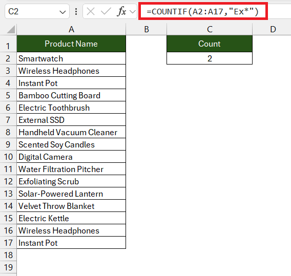
The asterisk (*) represents any number of characters. For example, if you want to count all products that start with “Ex” regardless of what follows, the criteria would be “Ex*”.
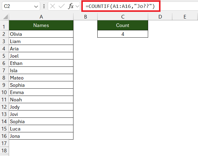
The question mark (?) replaces any single character. It’s great when you’re dealing with variations in spelling or missing letters, like finding all accounts where the name is four letters and starts with “Jo” – “Jo??”.
Lastly, the tilde (~) is a bit of an escape artist. When you actually need to find a literal asterisk, question mark, or tilde in your data, you precede it with a tilde. So, to find a value with an asterisk, your criteria would be “~*”.
Using wildcards can greatly enhance your counting capabilities in Excel by allowing nuances in your data to be easily summarized and understood.
Avoiding Double-Counting Pitfalls in Complex Formulas
When working with COUNTIFS across multiple criteria ranges, a common hazard is double-counting entries. This can happen if your criteria overlap or if you misuse cumulative COUNTIFS formulas. Pay special attention when counting unique occurrences in datasets with intersections.
Let’s say you’re evaluating a survey and counting how many times respondents chose “Agree” or “Strongly Agree” on different statements. A careless approach might lead you to simply add counts for each response, inadvertently inflating your totals if some responses span across both categories.
To avoid this pitfall, ensure your criteria are mutually exclusive or adjust your formula to exclude already counted responses. Sometimes, incorporating additional conditions or leveraging Excel’s SUMPRODUCT function alongside COUNTIFS can provide a more accurate count—especially if you’re dealing with multiple overlapping conditions.
Careful planning of your COUNTIF(S) strategies and a critical look at what you’re aiming to measure can go a long way in preventing double-counting and ensuring the reliability of your data analysis.
Troubleshooting Common COUNTIF Issues
Solving Syntax Errors: A Step-by-Step Guide
Syntax errors can be a common stumbling block when learning to use COUNTIF with more complex criteria. These errors arise when Excel doesn’t understand the command due to incorrect formula structure or arguments. Let’s troubleshoot together!
Firstly, double-check your formula’s structure: =COUNTIF(range, criteria). Ensure you’ve included the equals sign, range, and criteria, separated by a comma.
Next, inspect your range selection. It should be a continuous selection of cells, like A1:A10. Remember, if using COUNTIFS, all ranges must be the same size and shape.
Thirdly, review your criteria syntax. Text criteria need to be within quotes, like “Completed”. Numerical criteria or formulas, however, should not be enclosed in quotes unless they’re part of a text string, for example, “>10” or “<“&A1.
Also, ensure you’ve nested a standalone criterion within parentheses if it’s a part of a larger expression.
Lastly, if you’re using cell references in your criteria and encountering errors, verify those cells contain the correct data types and there are no leading or trailing spaces.
By methodically checking each element of your formula, you should be able to pinpoint and correct syntax errors, making your COUNTIF formula operational.
Overcoming COUNTIF’s Limitations with SUMPRODUCT
When your COUNTIF and COUNTIFS formulas hit their limits—whether it’s due to Excel’s restriction on the number of conditions or when trying to implement more complex logic—SUMPRODUCT emerges as a robust alternative. Unlike COUNTIFS, SUMPRODUCT can digest multi-layered conditions and tangled arrays without flinching.
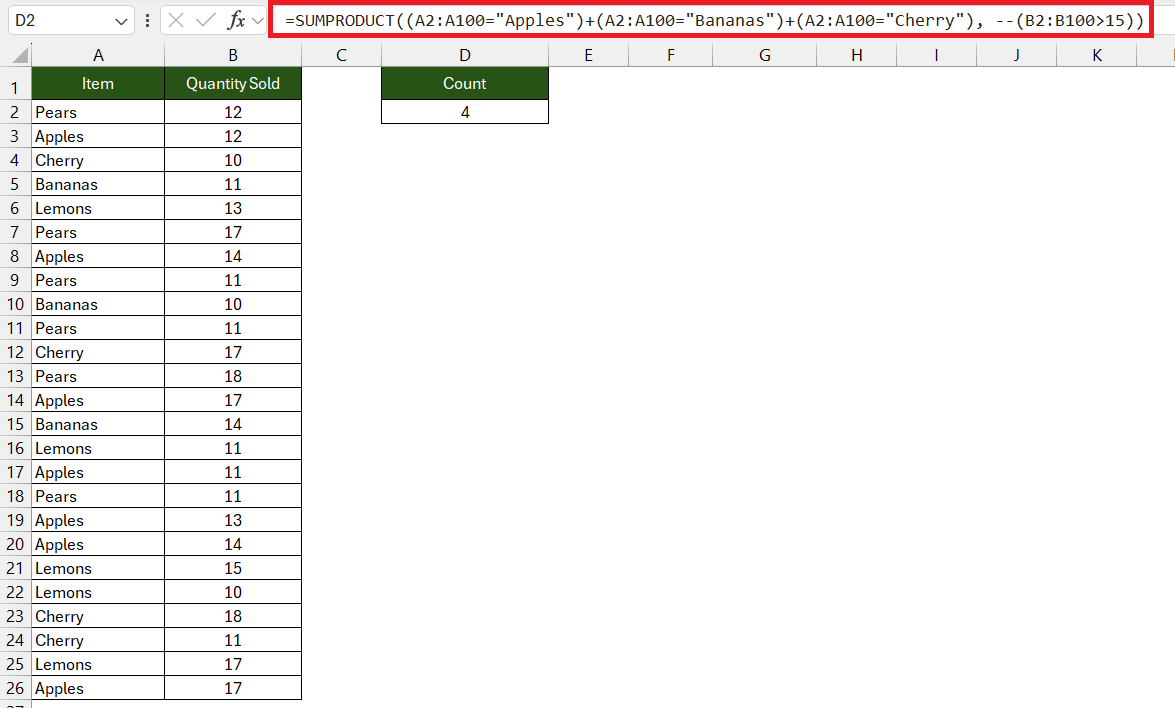
To illustrate, let’s revisit the task of counting rows that match various conditions with OR logic, which is tricky for COUNTIFS. Say you need to count all lines where the product is either “Apple,” “Banana,” or “Cherry” and the quantity sold is more than 15. SUMPRODUCT can elegantly tackle this:
=SUMPRODUCT((A2:A100="Apples")+(A2:A100="Bananas")+(A2:A100="Cherry"), --(B2:B100>15))
In this formula, SUMPRODUCT evaluates each condition against the range and returns an array of 1s and 0s. These are summed up, giving you the total count of rows meeting your criteria.
Mastering SUMPRODUCT opens a door to overcoming many of COUNTIF’s limitations, particularly when dealing with sophisticated data analysis needs.
FAQ: Expert Answers to Your COUNTIF Queries
How do I use COUNTIF with multiple conditions?
To use COUNTIF with multiple conditions in Excel, switch to the COUNTIFS function. Specify your ranges and each corresponding criterion. Here’s a quick formula example: =COUNTIFS(range1, criterion1, range2, criterion2). This way, Excel counts cells that meet all the criteria you’ve defined. Remember, each range-criterion pair is separated by a comma, and the function applies an AND logic to the conditions.
Can I combine AND and OR logic in one COUNTIF formula?
In native Excel functions, COUNTIF or COUNTIFS alone do not support combining AND and OR logic directly within a single formula. However, you can create a workaround by using multiple COUNTIFS for each set of OR conditions and summing the results for an AND combination. Alternatively, for more complex scenarios, the SUMPRODUCT function can accommodate both AND and OR logic by crafting arrays of conditions and summing the products. It requires a deeper understanding but offers a powerful solution when working with intricate data sets.
What are wildcard characters, and how do they work with COUNTIF?
Wildcard characters in Excel such as the asterisk (), question mark (?), and tilde (~) are used with COUNTIF to create flexible criteria for matching patterns of text. The asterisk () matches any sequence of characters, while the question mark (?) substitutes for a single character. Use the tilde (~) to search for the actual wildcard characters themselves. These are particularly useful when your text criteria are variable or partially known.
Can you add 2 Countifs together?
Yes, you can add two or more COUNTIFS functions together to count cells that meet any of the various criteria sets. This method often serves as a workaround for using OR logic, where you’re counting cells that match this criterion OR that criterion. You simply calculate each COUNTIFS separately and then add the results: =COUNTIFS(range1, criterion1) + COUNTIFS(range2, criterion2). This totals the counts from each condition.
Can you do a Countif with multiple criteria sheets?
Absolutely, you can use COUNTIF or COUNTIFS across multiple sheets in Excel. When you define your range, you’ll just need to include the sheet name followed by an exclamation point before the cell range. For example: =COUNTIFS(Sheet1!A:A, criterion1, Sheet2!B:B, criterion2). This formula will count cells that meet criterion1 on Sheet1 and criterion2 on Sheet2.
John Michaloudis is a former accountant and finance analyst at General Electric, a Microsoft MVP since 2020, an Amazon #1 bestselling author of 4 Microsoft Excel books and teacher of Microsoft Excel & Office over at his flagship Academy Online Course.
