How to Use the COUNTIFS Function in Microsoft Excel

In this article, we will be looking at how to use the COUNTIFS function in Excel. The COUNTIFS function in Excel is an extremely useful tool when you want to count things based on multiple conditions or criteria.

Syntax:

=COUNTIFS(range1, criteria1,[range2], [criteria2],…)

COUNTIFS: The name of the function

range1, range2:  The ranges of cells where Excel will look for the data. Multiple ranges can be separated by commas. Each range represents a column or a group of cells in your table.

criteria1, criteria2:  The conditions or criteria that Excel will use to determine which items to count. You provide one criteria for each range. Each criterion can be a value, a cell reference, a text string, or a logical expression.

(Remember that you can use up to 127 range and criteria pairs in COUNTIFS. Now, that’s powerful!)

We will explore several parts of this formula:

• Basic Application
• Cell References
• COUNTIFS with logical criteria
• Wildcards

Let’s look at these methods thoroughly!

Download the Excel Workbook below to follow along and understand How to Use the COUNTIFS Function in Microsoft Excel –

download excel workbookCOUNTIFS.xlsx

Basic Application

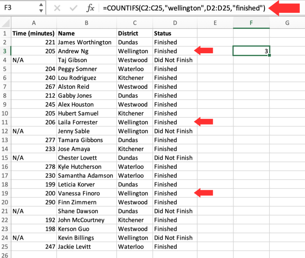
Let’s say you have a table containing the results of a marathon race. Column A contains the time the competitors finished, column B contains the names of the competitors, column C is their respective districts, and column D is whether they completed the race or did not complete the race. We will use 2 range and criteria for this example.

We want to find out how many competitors from the Wellington district finished the race.

The formula will be:

=COUNTIFS(C2:C25,”wellington”,D2:D25,”finished”)

First criteria: C2:C25 range. The criteria we want them to meet is that they should be from the Wellington region. Since it is a text value, we enclose that within double quotes.

Second criteria: D2:D25 range. We want to know how how many of them finished the race.

As you can see the results return as 3. Meaning 3 racers from the Wellington region finished the race.

Cell References

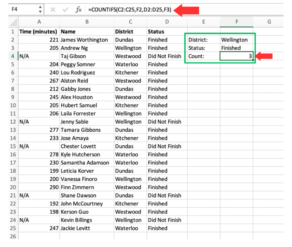
In that example, we used the hardcoded values as part of the formula. But, it is usually better to use cell references for flexibility reasons. If we use cell references, we do not have to change the formula whenever we change the values entered in the input cell.

Here’s how it’s done:

District: Wellington

Status: Finished

Count: =COUNTIFS(C2:C25,F2,D2:D25,F3)

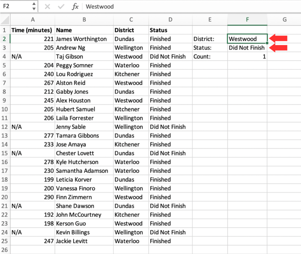
As you can see, we get the same results as the hardcoded values. But, the big advantage is that we can change the criteria easily without having to change the formula.

COUNTIFS with logical criteria

The COUNTIFS function allows us to count not just exact matches but also include cells that are greater than, less than, or not equal to certain values. By using logical operators like > (greater than), < (less than), and = (equal to), we can specify criteria to identify cells with values within a specific range.

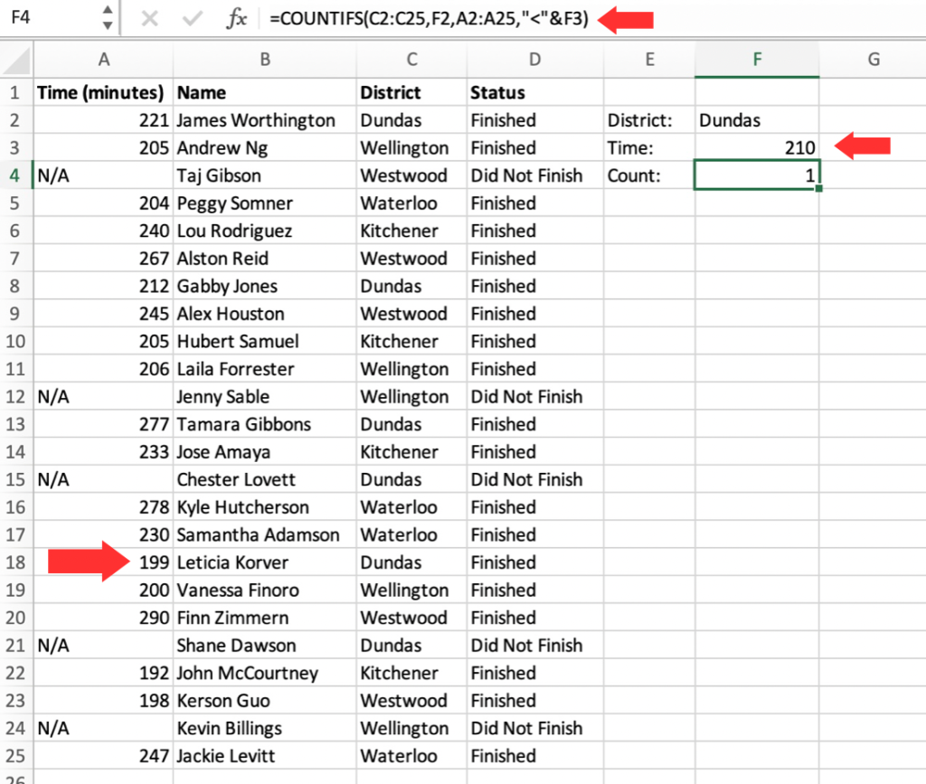
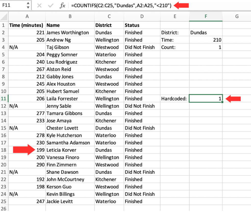
For example, the formula below can be used to count the number of racers from the Dundas district who completed the race under 3.5 hours.

=COUNTIFS(C2:C25,F2,A2:A25,”<“&F3)

As you can see, the results returned only one person (Leticia Korver) from the Dundas district who ran the race under 3.5 hours.

If we did not want to use cell references, and wanted to use hardcoded values instead, we can use this formula:

=COUNTIFS(C2:C25,”Dundas”,A2:A25,”<210”)

 

Wildcards

When it comes to summarizing data, we often encounter a challenge where the data we want to count is similar but not exactly the same. However, a great alternative to overcome this issue is to use WILDCARDS. Thankfully, the COUNTIFS function in Excel supports the use of wildcards, allowing us to perform counts with partial matches.

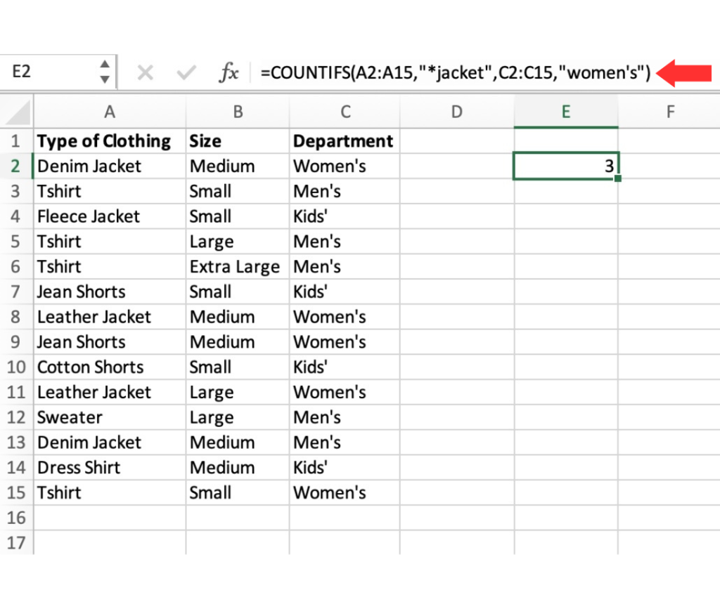
For example, we want to count the number of jackets in the women’s department. The problem is, there are several types of jackets like denim, fleece, and leather listed in the inventory. We can use the asterisk sign (*) before the word “jacket”

Let’s use this formula:

=COUNTIFS(A2:A15,”*jacket”,C2:C15,”women’s”)

You can include wildcard characters such as the question mark (?), asterisk (*), or tilde (~) in your criteria when using the COUNTIFS function. The question mark (?) can be used to represent any single character, while the asterisk (*) can represent zero or more characters of any kind.

The tilde (~) serves as an escape character, enabling you to search for wildcard characters as literal characters within the COUNTIFS function.

There you have it! The COUNTIFS function gets rid of the necessity to create complex formulas or pivot tables for answering simple questions. Its syntax is straightforward to understand, and its ability to work with wildcards adds an extra advantage.