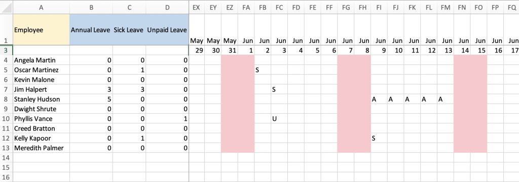
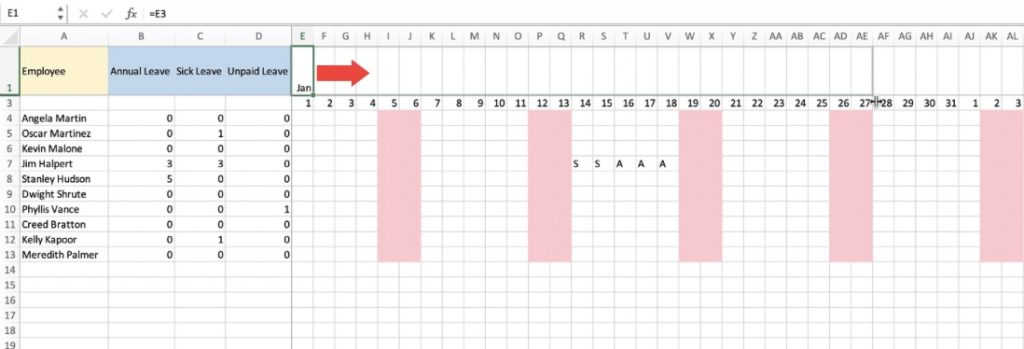
Managing employee leave records is an important aspect of human resource management for any company. Having a well-organized and comprehensive leave record in Excel can help businesses keep track of employee absences and maintain transparency. In this article, we’ll guide you through the process of how to create a yearly leave record for employees in Excel. The final spreadsheet would look something like this:
Let’s explore these methods!
Download the Excel Workbook below to follow along and understand How to Create A Yearly Leave Record for Employees in Excel –
Download excel workbookYearlyLeaveRecord1.xlsx
Planning Your Spreadsheet
Before diving into Excel, it’s essential to plan how you want to structure your employee’s yearly leave record.
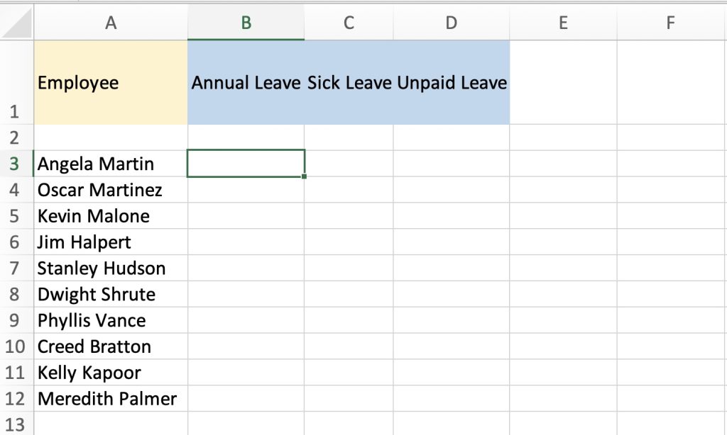
Employee Information: Decide on the employee details you want to include, such as employee name, ID, department, or contact information. In our case we’ll use the employee names.
Leave Types: Identify the types of leave you want to track, such as annual leave, sick leave, and unpaid leave.
Open Excel and create a new workbook.
In the first row of your spreadsheet, set up the headers:
– Employee Name
– Leave Type (Annual Leave, Sick Leave, and Unpaid Leave)
You can customize these headers based on your organization’s needs.
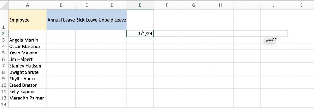
In cell E2, input the date 1/1/2024.
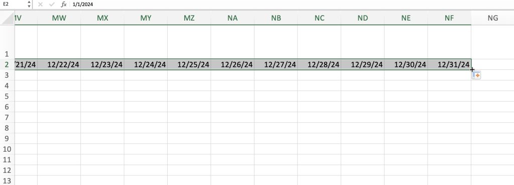
Click and drag the square on the bottom-right of the cell to apply this date format to the rest of the columns until you reach the end of the year (12/31/2024.) This will lead you to column NF.
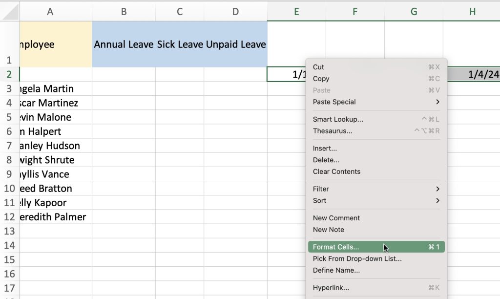
Highlight all of the dates. Then, right-click to select Format Cells.
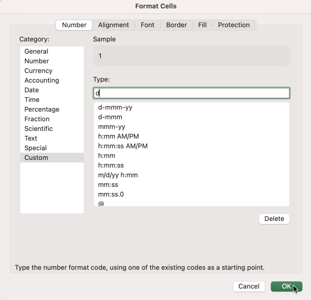
From the Format Cells Menu, click on Custom and select “d” to show the day of the month.
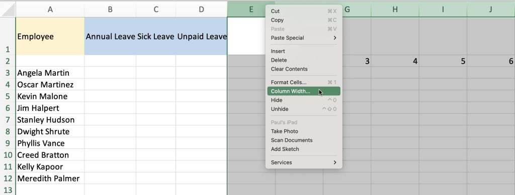
At this point, we would like to make the columns more compact for ease of use. Highlight the columns from E to NF then right-click. Select Column Width, type in 3 and click OK.
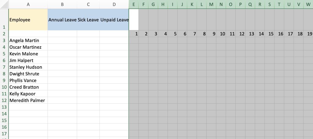
As you can see, the columns are now more compact.
Using the WEEKDAY Function
Next up, we would like to mark the weekends (or the days when the employees are not working) on our calendar and fill the those cells with the color red.
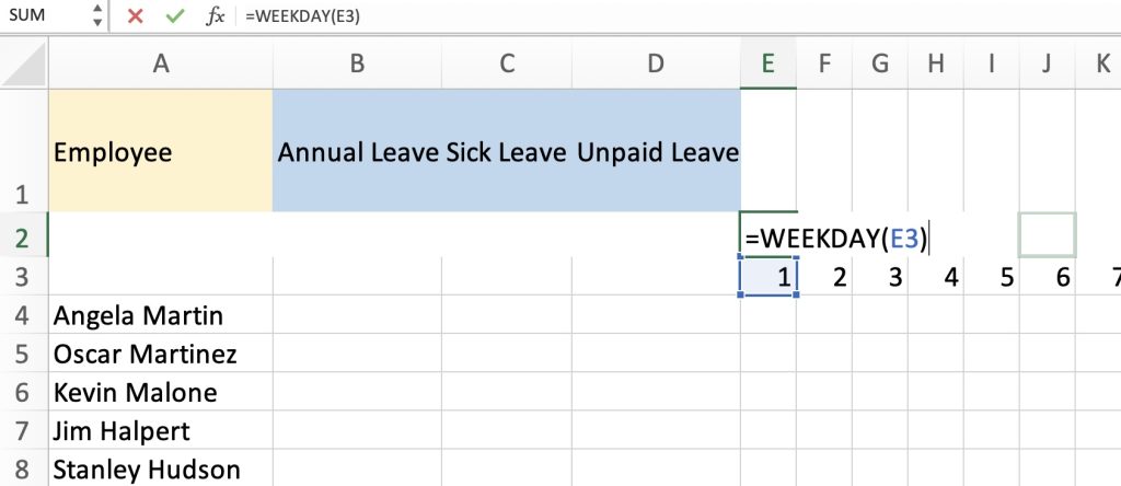
Right-click to Insert a new row above the dates.
Select cell E2, enter the formula =WEEKDAY(E3)
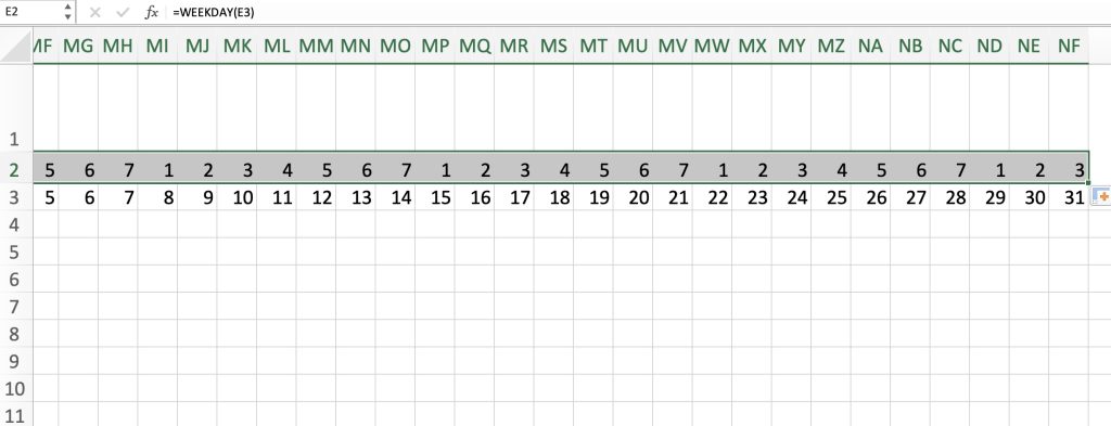
Note: In Microsoft, Saturdays are bound to 7, Sundays are 1, Mondays are 2, etc. The number on cell E2 is a 2 because January 1st is on a Monday.
Drag the formula to the end of the year.
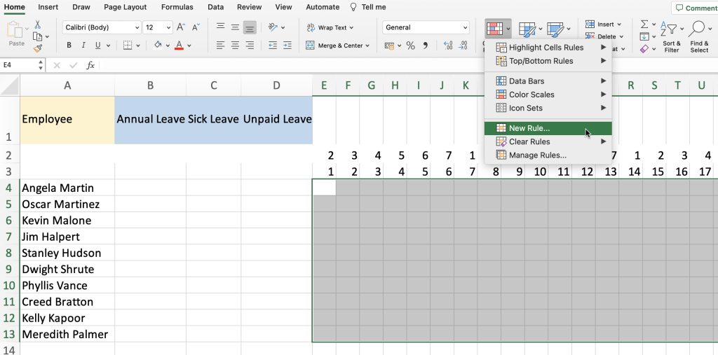
Highlight cells E4 to NF13. Go up to Conditional Formatting and select New Rule.
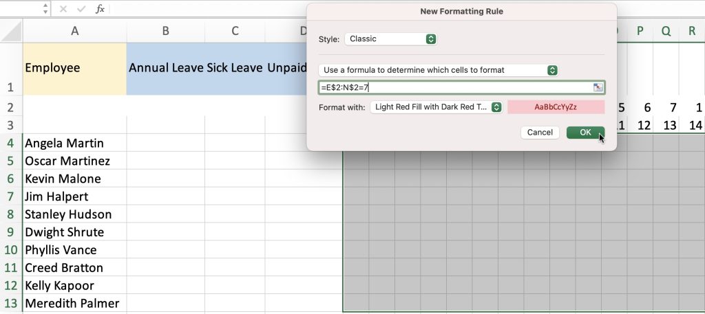
Choose “Use a formula to determine which cells to format.”
Enter this formula: =E$2:N$2=6 (6 represents Saturday)
Select Format.
Go to Fill and select the color red.
Repeat the same steps for Sunday. This time, the formula will be: =E$2:N$2=7
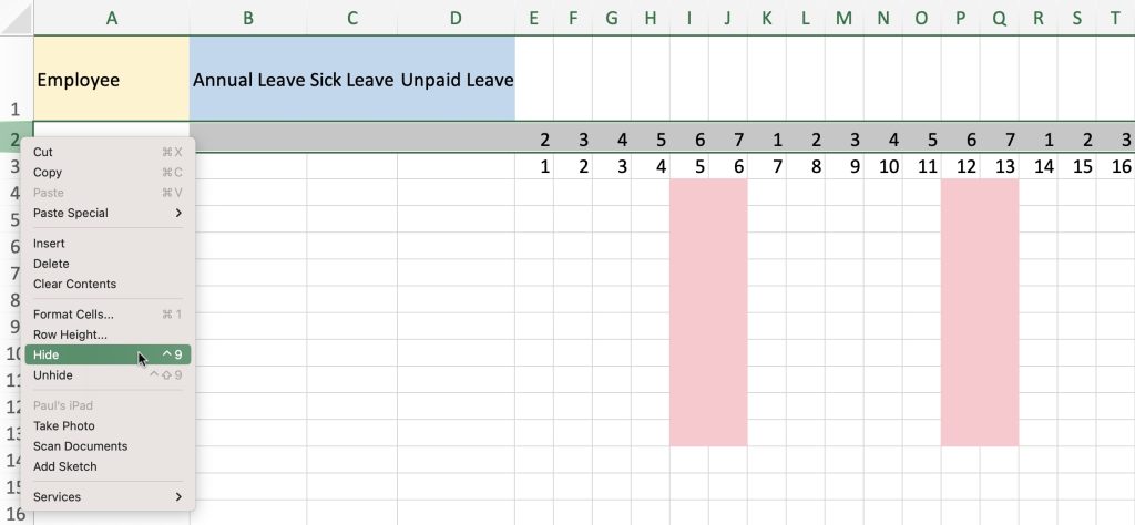
Now that we have the weekends marked off, we can right-click row 2 and select Hide.
Click here to learn more about Excel Date and Time Functions!
Using the COUNTIF Function
At this stage, we will use the COUNTIF formula to tally the amount of sick leaves, annual leaves, and unpaid leaves an employee uses throughout the year.
Example: Kevin Malone uses a Sick Leave on the 2nd of January. HR will jot down January 2nd with a simple “S” and the formula will automatically add 1 to his Sick Leave tally.
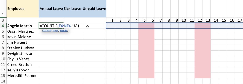
Select cell B4, and enter the formula: =COUNTIF(E4:NF4,”A”)
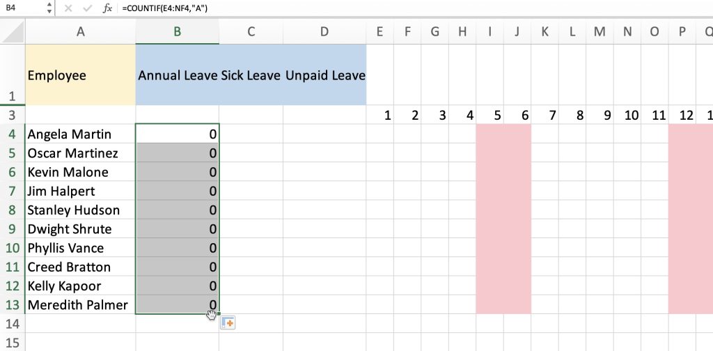
Drag the formula down for the rest of the employees.
Use the same formula for Annual Leaves, and Unpaid Leaves. Only this time, using the letters “S” and “U” as distinctions.
=COUNTIF(E4:NF4,”S”)
=COUNTIF(E4:NF4,”U”)
Click here to learn more about the COUNTIF Function!
Formatting the Months
Now let’s mark the months to make the data sheet more manageable.
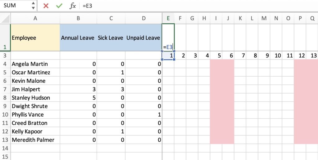
Select the cell just above the first day of January.
Enter =E3
Right-click and go to Format.
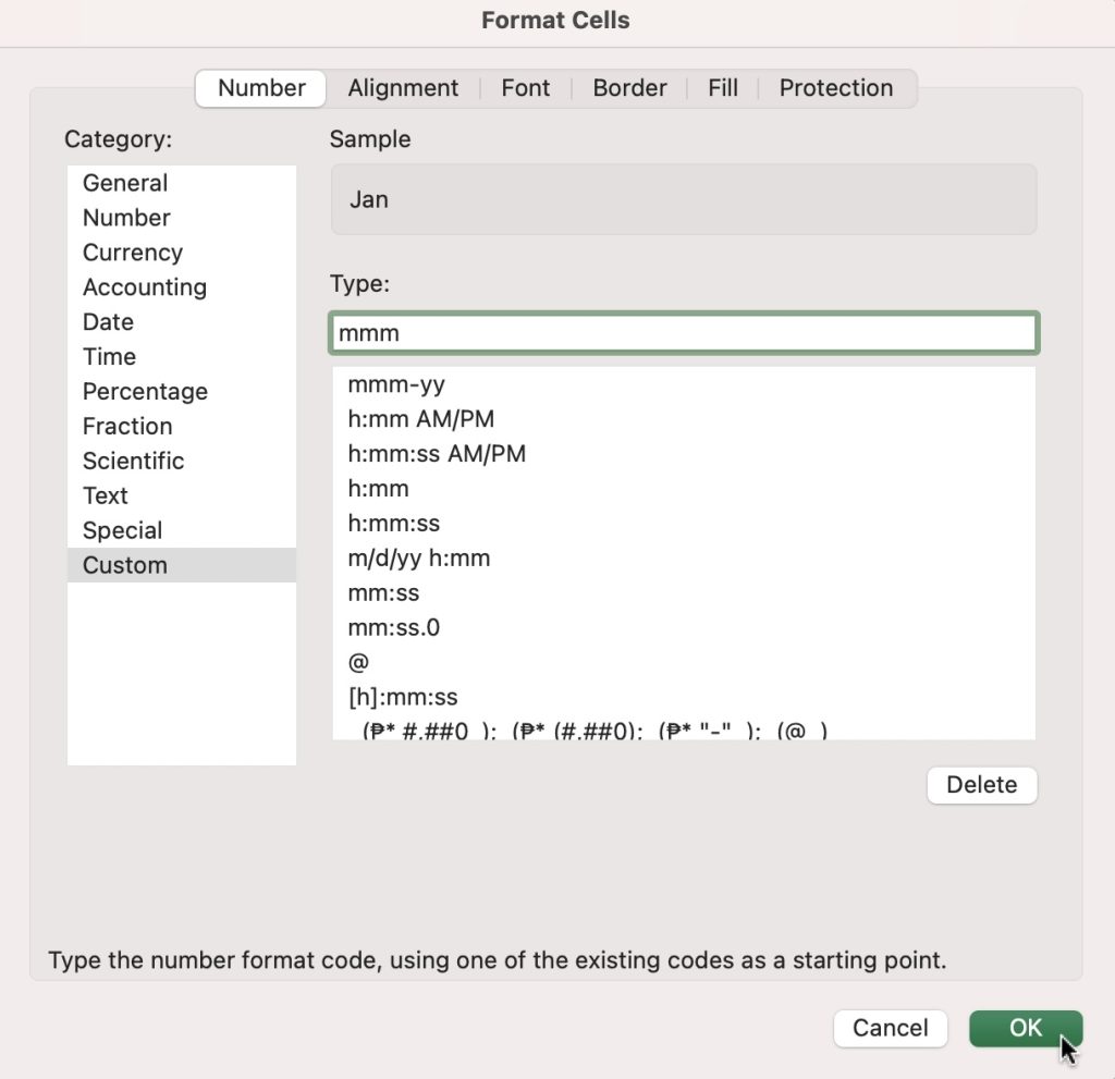
On the Number tab, select Custom and type in “mmm”
This will give you the first 3 letters of the month.
Click and drag the square on the bottom-right of cell E6 to apply the formula to the rest of the months.
Click here to master Custom Formatting in Excel!
Freeze Pane
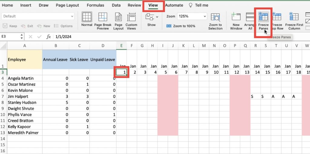
One of the neat things about Excel is you can utilize Freeze Pane to ensure that the header row or column remains visible, even when scrolling. This is particularly helpful when you need navigate and input data in a large spreadsheet.
Select cell E3, go to the View tab, and select Freeze Panes.
Now, you’ll be able to scroll all the way across the spreadsheet.
Conclusion:
There you have it! Creating an employee yearly leave record format in Excel will help you become more organized in your workforce management. Make sure to use these steps for your 2024 Employee Leave Record!
Click here to access Microsoft’s tutorial on How to Use the COUNTIF Function!
John Michaloudis is a former accountant and finance analyst at General Electric, a Microsoft MVP since 2020, an Amazon #1 bestselling author of 4 Microsoft Excel books and teacher of Microsoft Excel & Office over at his flagship Academy Online Course.
