What does it do?
It returns a reference to a range, from a starting point to a specified number of rows, columns, height and width of cells
Formula breakdown:
=OFFSET(reference, rows, columns, [height], [width])
What it means:
=OFFSET(start in this cell, go up/down a number of rows, go left/right a number of columns, height of range, width of range)
The OFFSET function in Excel is one of the Lookup functions and is great if you want to reference a range of cells and use that reference to do a calculation.
Click here to see how the formula works visually & interactively
When we have a large data set and add new rows/columns of data on a daily basis, we sometimes want to capture that new data in our analysis automatically without having to amend the data range.
One example is when we are using a Pivot Table and our data source is not in an Excel Table. We want the new data to be added in the Pivot Table’s Data Source automatically without having to Change the Data Source each time manually.
This is how it is done below (go to the bottom of the page if you want to see the animated gif tutorial):
Download excel workbookOffset-Dynamic-Data-Range.xlsx
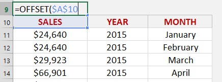
STEP 1: We need to enter the Offset function
Table of Contents
=OFFSET
STEP 2: 1st Offset argument – Where do we want to to start our reference?
This is at the start of the data source (i.e. the top left hand corner)
Make sure to add an absolute reference to the 1st argument by pressing F4
=OFFSET($A$10
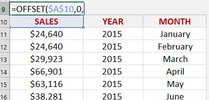
STEP 3: 2nd Offset argument – How many Rows down do we want to go?
As we want the referenced range to start at cell A10, we simply enter 0
=OFFSET($A$10, 0,
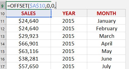
STEP 4: 3rd Offset argument – How many Columns to the right/left do we want to move?
We do not want to move to any Columns, so we simply enter 0
=OFFSET($A$10, 0,0,
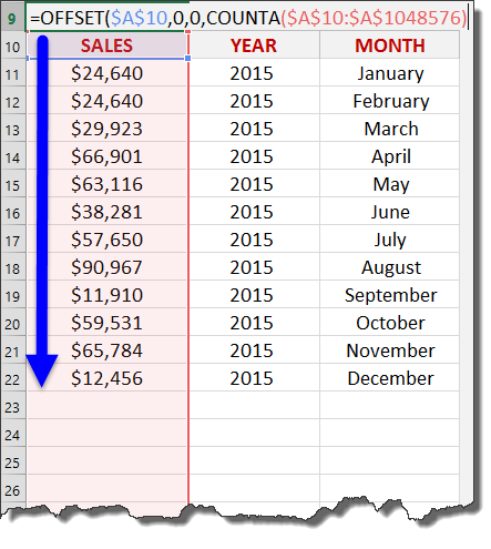
STEP 5: 4th Offset argument – How High do we want our referenced data to be?
This is where the COUNTA function is used to count how many transactions we have in our data vertically and return the [height] of our data.
So as we are starting at cell A10, we are going to capture 13 cells downwards ( COUNTA(A10:A1048576) ) i.e. The range up to the last active vertical cell of our data.
NB: It is always a good idea to enter an ending range that is more than your last data cell or up till the last row number i.e. 1,048,756. That way as your new data get entered, we will be sure to capture it!
Make sure to add an absolute reference to the 4th argument by pressing F4
=OFFSET($A$10, 0,0,COUNTA($A$10:$A$1048576
STEP 6: 5th Offset argument – How Wide do we want our referenced data to be?
This is where the COUNTA function is used to count how many transactions we have in our data horizontally and return the [width] of our data.
So as we are starting at cell A10, we are going to capture 3 cells to the right( COUNTA($A$10:$XFC$10) ) i.e. The range up to the last active horizontal cell of our data.
NB: It is always a good idea to enter an ending range that is more than your last data cell or up till the last column number i.e. XFC. That way as your new data get entered, we will be sure to capture it!
Make sure to add an absolute reference to the 4th argument by pressing F4
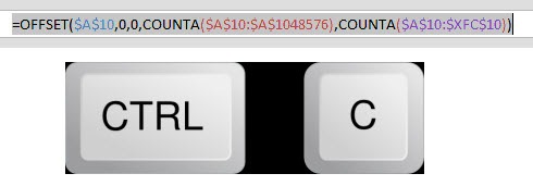
=OFFSET($A$10, 0,0,COUNTA($A$10:$A$1048576,),COUNTA($A$10:$XFC$10))
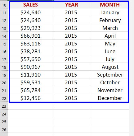
As you can see from the image below, the OFFSET function captures the following data range:
STEP 7: Now that we have our OFFSET function, we need to create a Named Range for it so we can use it as our data source in Step 9.
To do this we need to select the whole OFFSET function and Copy it…
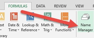
…and go to Formulas > Name Manager > New:
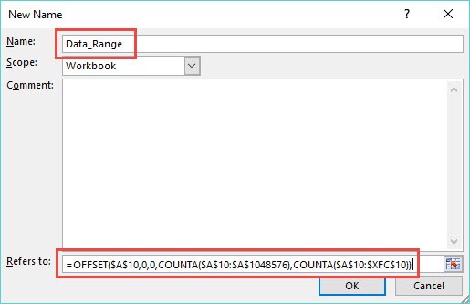
STEP 8: In the New Name dialogue box we need to enter a custom name with no spaces e.g. Data_Range in the Name: area and paste the OFFSET function from Step 7 in the Refers to: area and press OK
STEP 9: We need to insert a Pivot Table by going to Insert > Pivot Table…
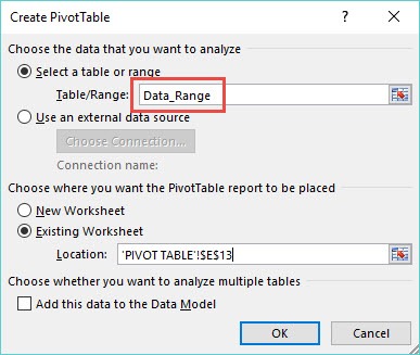
…and in the Create PivotTable dialogue box we need to manually enter the Named Range from Step 8 i.e. Data_Range into the Table/Range area, choose a New/Existing Worksheet and press OK:
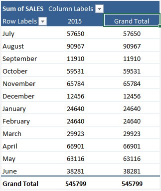
STEP 10: In the Pivot Table, you will need to put the SALES field in the VALUES area, the YEAR field in the COLUMNS area and the MONTH field in the ROW area:
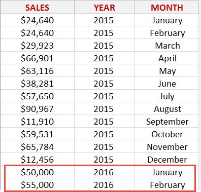
STEP 11: In your data source you can start adding new data in the empty rows:
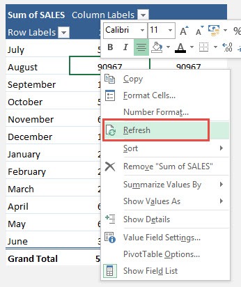
STEP 12: To reflect this new data in the Pivot Table, all you need to do is Right Click inside the Pivot Table and choose Refresh:
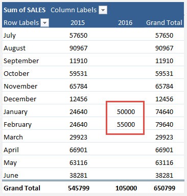
The new data will now be shown in the Pivot Table:
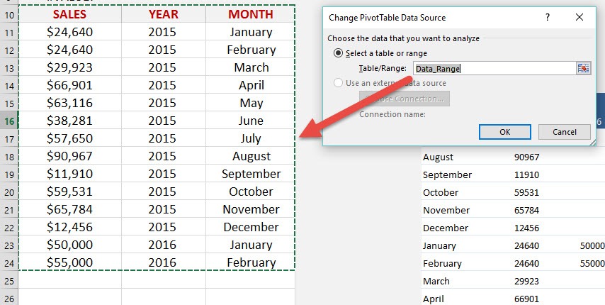
STEP 13: To check that our Named Range called Data_Range captures the new data entered, we need to click in the Pivot Table and go to PivotTable Tools >Analyze/Options > Change Data Source:
So we can confirm that our Named Range Data_Range captures any new data entered in our data source!
This is a great trick but if you use an Excel Table as your data source, you avoid creating this OFFSET function within a Named Range. Excel Tables rock but Excel purists still love playing around with formulas, so this trick is for you 🙂
John Michaloudis is a former accountant and finance analyst at General Electric, a Microsoft MVP since 2020, an Amazon #1 bestselling author of 4 Microsoft Excel books and teacher of Microsoft Excel & Office over at his flagship Academy Online Course.

