Excel 2016 Histogram Charts are one of the many new Charts available only in Excel 2016.
They are very visual as it can easily show you the distribution of numerical data, like seeing which numerical ranges are the most common.
In this article, we will discuss the following:
What is a Histogram?
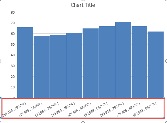
Histogram is a graphical representation of data that shows frequency distribution i.e. count of data in a specified range.
It looks like a column chart where each column or bar represents a specific range and its height determines the frequency or count of that range.
For example, you can use the histogram to display the count of sales between different sales ranges like $0-$500, $500-$1000, $1000-$1500, $1500-$2000, and so on.
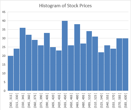
This is how an Excel 2016 Histogram looks like this:
Now that you are familiar with what a histogram is, let’s move forward and learn how to create a Histogram in Excel 2016.
How to Create a Histogram in Excel?
You can create a Histogram in different ways described below:
- In Excel 2016 using a Built-in Histogram Chart Option.
- In Excel 2013 or prior version, using a Data Analysis Toolpack.
- Using Frequency function
Using Built-in Histogram Chart Option (In Excel 2016)
In this example, I show you How to Make a Histogram in Excel 2016.
To upgrade to Excel 2016 you can use this link here: Microsoft Office 2016
Follow the step-by-step tutorial on How to Create a Histogram in Excel 2016 with its built-in option available.
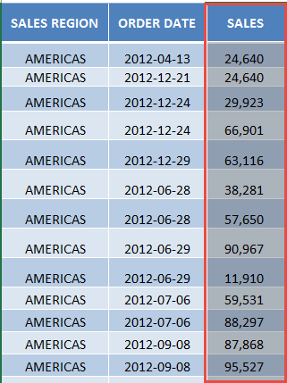
STEP 1: Highlight your column with numerical data.
STEP 2: Go to Insert > Recommended Charts
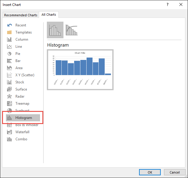
STEP 3: In the Insert Chart dialog box, Select All Charts > Histogram > OK
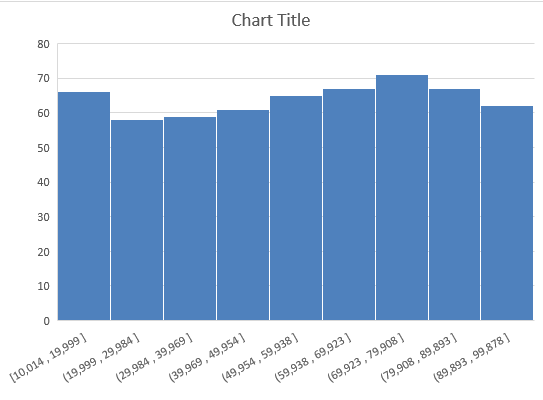
STEP 4: Now you have your Histogram Chart.
You can easily change the way how your Histogram Chart represents your data, by following the steps below:
STEP 1: Double-clicking on the horizontal axis containing our values.
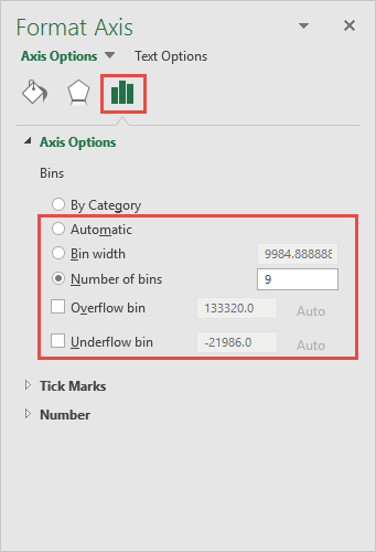
STEP 2: In the Format Axis window, pick the third option Axis Options. Let us go through the options you can use:
Automatic – Excel does the heavy lifting for you, and determines what the size of each bin would be.
Bin width – You tell Excel how many units each bin should be. In our example below, we are telling Excel that we want each bin to cover 9,984 units each.
Number of bins – Excel will automatically determine the size of each bin, however, you can modify the number of bins.
Overflow bin – This will set a threshold for your bins, any value above this threshold will be placed in this bin.
Underflow bin – This will set a threshold for your bins, any value below this threshold will be placed in this bin.
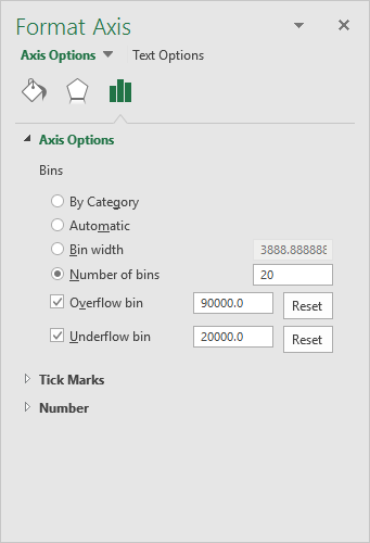
STEP 3: Try out the following settings to modify the Excel 2016 Histogram Chart:
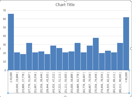
Number of Bins – 20
Overflow Bin – 90,000
Underflow Bin – 20,000
Now you have your cool Histogram chart and you can quickly point out to your management which range of values are the most common ones…
Using Data Analysis Toolpack (In Excel 2013 or prior version)
Since the built-in histogram option is not available in Excel 2013 or the prior versions, you can create a Histogram using the Data Analysis Toolpack.
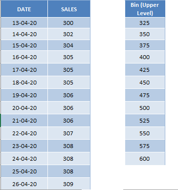
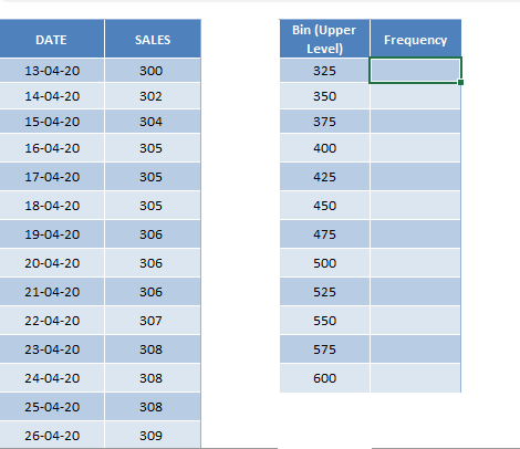
In the data table, you have a daily stock price listed and the range (upper level) below:
Let’s see how to create a histogram of the daily stock price reported!
STEP 1: Go to Data Tab > Data Analysis
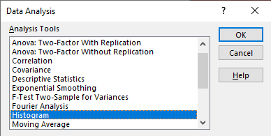
STEP 2: In the Data Analysis dialog box, Select Histogram > Press OK.
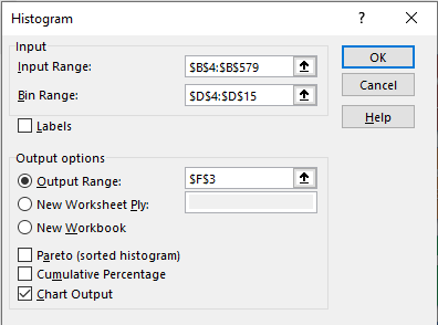
STEP 3: In the Histogram dialog box, enter the Input Range as $B$4:$B$579, Bin Range as $D$4:$D$15, Output Range as $F$3 and lastly make sure to check Chart Output.
Press OK.
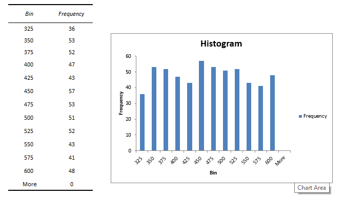
Your Histogram Chart is ready!
You can change the format of this Chart by following the steps below:
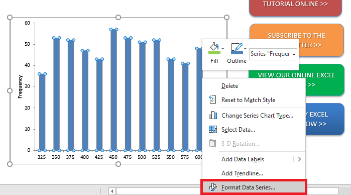
STEP 1: Right Click on the bar and select Format Data Series.
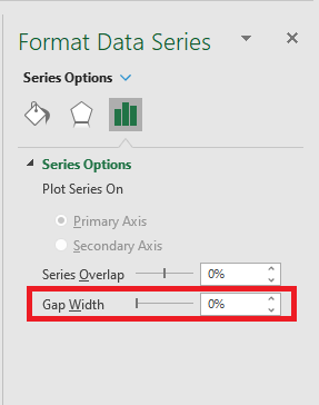
STEP 2: In the Format Data Series dialog box, change the Gap width from 150% to 0%.
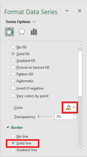
STEP 3: Click on the Fill icon, change the color of the bar, and add a solid border line.
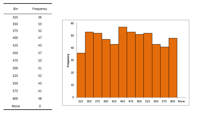
Your formatted Histogram in Excel is ready!
The two ways that you saw earlier can easily help you create a histogram but they will not be dynamic i.e. they will not update once you change the data.
To make a dynamic Histogram, you can use a FREQUENCY function in Excel.
FREQUENCY function in Excel is used to calculate how often values occur within a range of values. This function has two arguments – Data Array and Bins Array.
- Data_Array: Range for which you get the frequencies.
- Bins_Array: Range containing intervals or upper-level bins.
You can use the Frequency to calculate how many values fall in the specified ranges and then create a column chart using that data.
Let’s take the same example of the distribution of daily stock prices as above and see how the Frequency function works to create a Histogram.
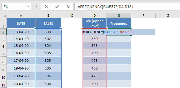
STEP 1: Insert formula to be used will be =FREQUENCY(B4:B579, D4:D15).
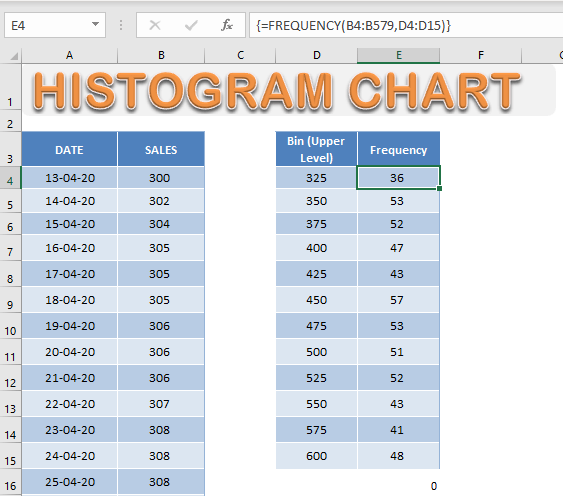
STEP 2: Make sure to press Ctrl + Shift + Enter to complete the function and then copy-paste the formula below.
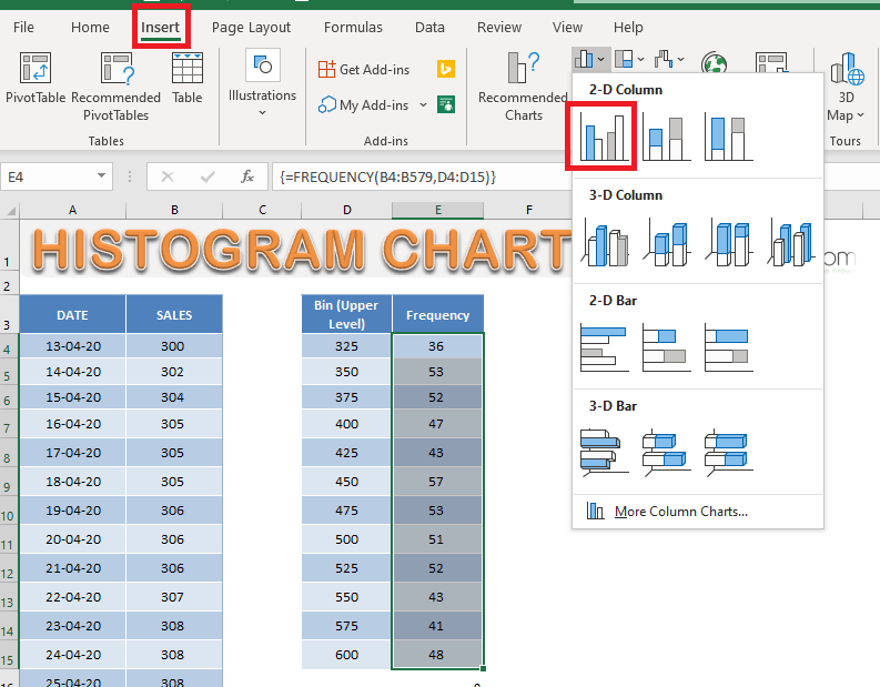
STEP 3: Select the Frequency Column and the Go to Insert > Column Chart.
STEP 4: Go to Chart Design > Select Data.
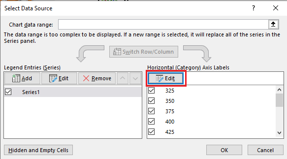
STEP 5: In the Select Data Source dialog box, Under Horizontal (Category) Axis Label select Edit.
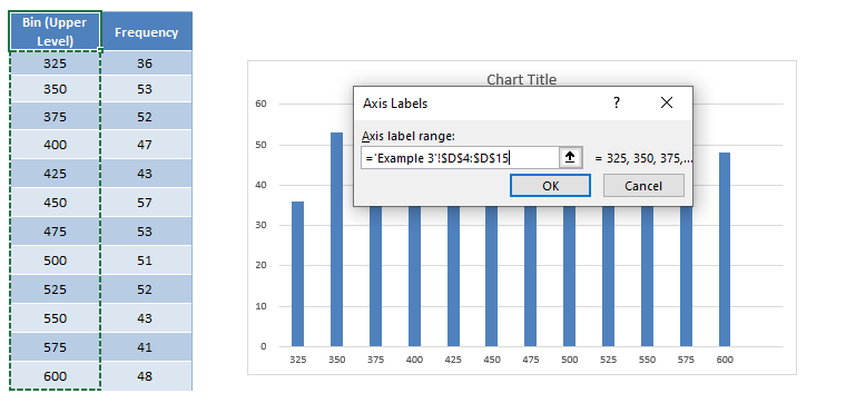
STEP 6: Select the range containing the bin value i.e. D4:D15 and then Click OK.
Your dynamic Histogram 2016 Excel chart is ready!
Conclusion
A Histogram Excel 2016 can be used to show the number of data that fall within a specified range of values (bins).
In this article, you have learned How to Create a Histogram in Excel using the built-in option, the data analysis toolpack, and the frequency function.
To read about the other charts available in Excel, Click Here.
HELPFUL RESOURCE:
Bryan
Bryan is a best-selling book author of the 101 Excel Series paperback books.
