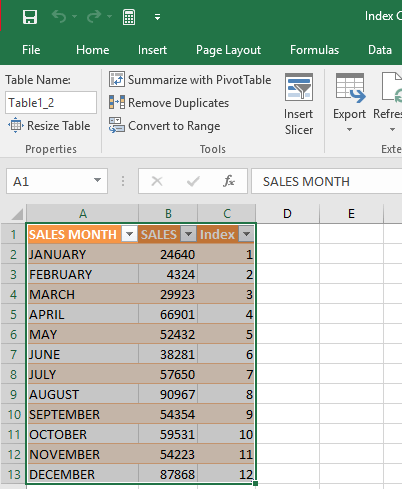
Power Query lets you perform a series of steps to transform your Excel data. One of the most common steps I do, is I want to add an index column that serves as a row counter of my data.
There is the alternative method of using the ROW formula in Excel.
However if we simply want to keep it as a temporary column for data analysis, we can generate the Row Numbers using Power Query.
Thankfully Power Query has an option that allows us to create Index Columns!
Let’s go through the steps in detail:
STEP 1: Our sample data consists of Months and multiple Sales values for each quarter. Let us say we want a column that counts from 1 to 12 next to our data to serve as our row numbers.
(Make sure that your data is firstly converted into an Excel Table by pressing CTRL+T and OK).
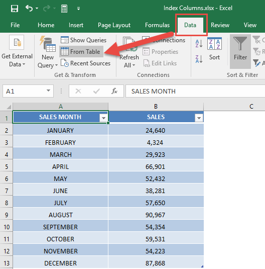
Go to Data > Get & Transform > From Table (Excel 2016) or Power Query > Excel Data > From Table (Excel 2013 & 2010)
Excel 2016:
Excel 2013 & 2010:
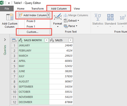
STEP 2: This will open up the Power Query Editor.
Within here you need to select Add Column > Add Index Column > Custom
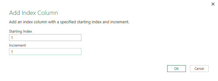
STEP 3: This brings up the Index Column dialogue box.
Set the Starting Index into 1, this would mean the starting number will be 1.
For the Increment, place in 1. This means that every succeeding number will be incremented by one. So we will have 1, 2, 3, 4 and so on..
Click OK.
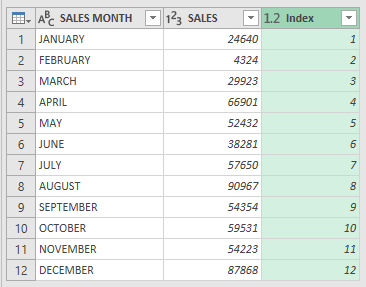
STEP 4: Now you will see your changes take place and the data now has an index column!
STEP 5: Click Close & Load from the Home tab and this will automatically open up a brand new worksheet in your Excel workbook with the new data.
You now have your new table with your index column!
HELPFUL RESOURCE:
Bryan
Bryan is a best-selling book author of the 101 Excel Series paperback books.
