In this article, we’ll explore two effective methods for achieving this advanced data consolidation within Excel –
Let’s explore these methods!
Download the Excel Workbook below to follow along and understand How to Create PivotTable from Multiple Sheets in Excel –
download excel workbookPivot-Table-from-Multiple-Sheets-1.xlsx
Method 1 – Pivot Table Wizard
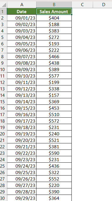
Suppose you have sales data from two different locations – West and East. You want to create a Pivot Table that will show the sum of sales from both locations combined in a single report. Follow the steps below to create PivotTable from multiple sheets –
STEP 1: Press Alt + D + P to open the PivotTable Wizard.
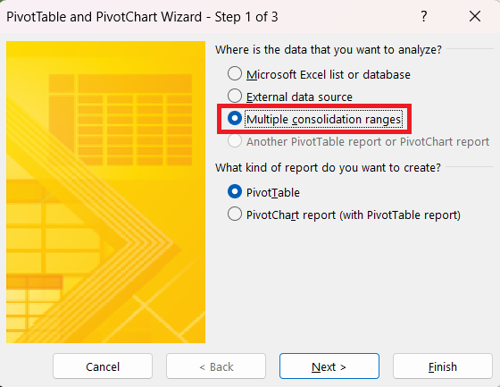
STEP 2: In the PivotTable and PivotChart Wizard, select Multiple consolidation ranges and press Next.
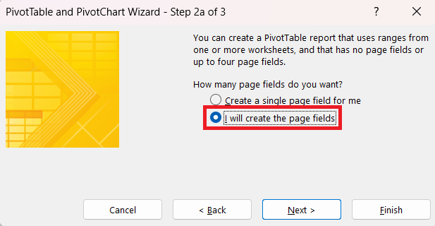
STEP 3: Select I will create the page fields option and then Next.
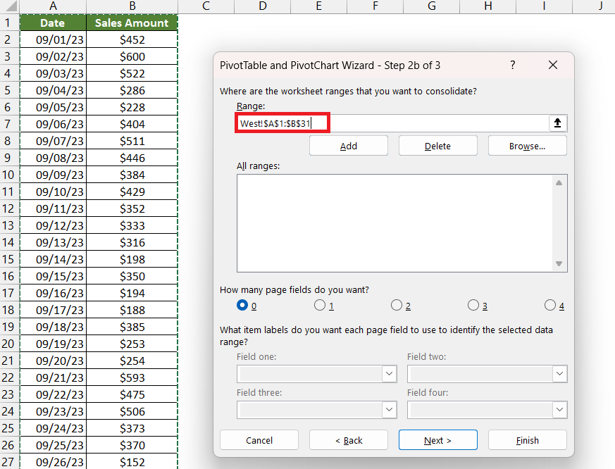
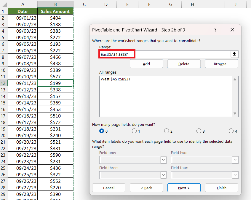
STEP 4: Select the data table from the West region and click Add.
STEP 5: Select the data table from the East region and click Add.
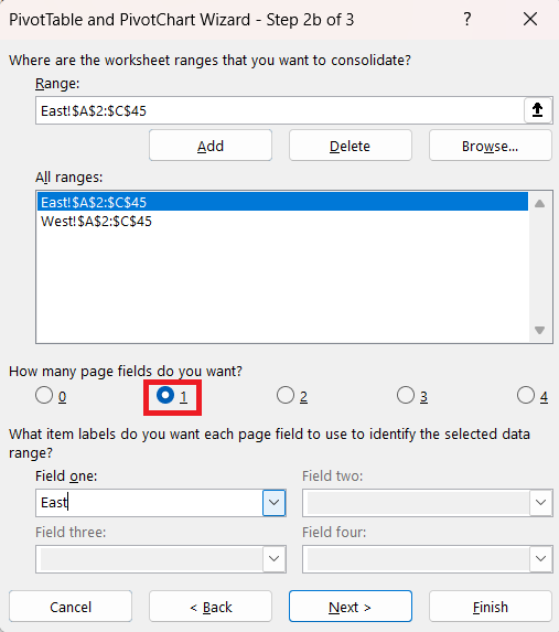
STEP 6: Select 1 as the page field.
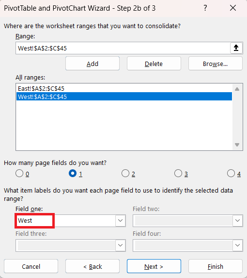
STEP 7: Select the range of the West region and type West in the Field one box.
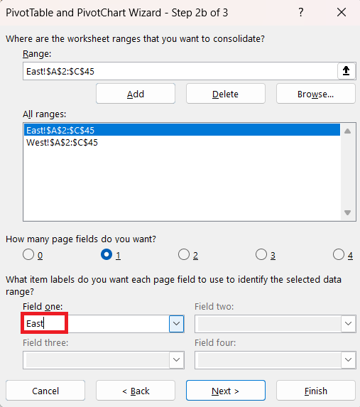
STEP 8: Select the range of the East region and type East in the Field one box. Click Next.
STEP 9: Select New Worksheet. Click Finish.
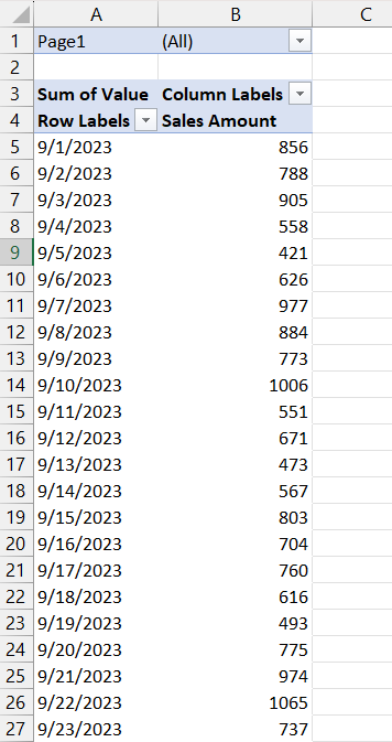
A PivotTable combining data from both sheets will be displayed in the new worksheet.
Method 2 – Using PowerQuery
In this method, you can add data from different sheets into a single data table and then use it to create Pivot. You can do this using the append queries option in Power Query. Power Query can append or merge two separate tables together as well as create extra columns in your data which can display your custom calculations.
The Power Query method grants extensive flexibility and control over the data consolidation process. Follow the steps below to create a PivotTable from multiple sheets –
STEP 1: Go to Data > From Table/Range.
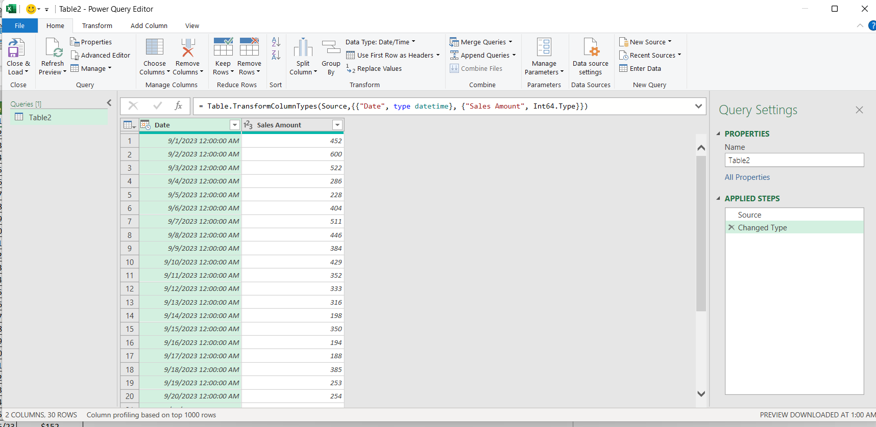
The data table will now open in the Power Query editor window.
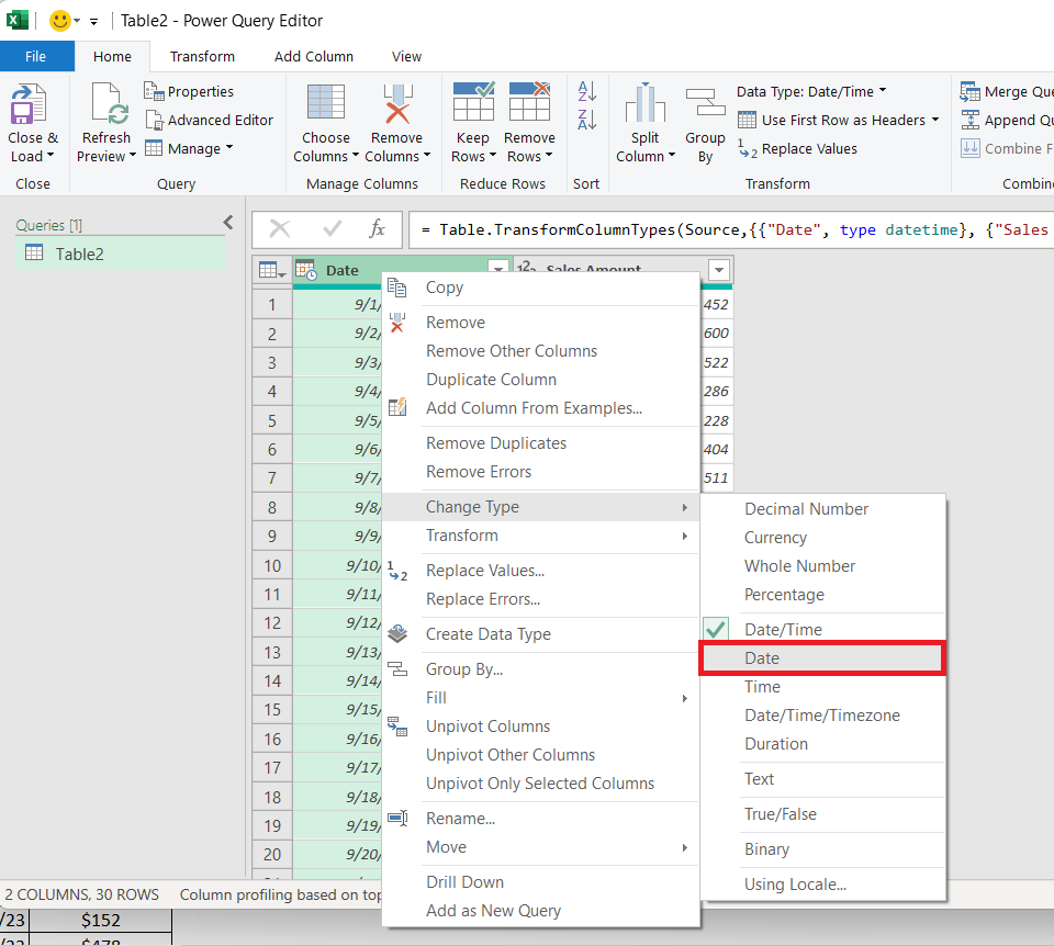
STEP 2: Right-click on the date column and select Change Type > Date.
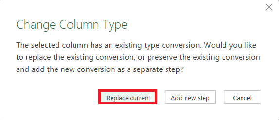
STEP 3: In the Change column type dialog box, select Replace current.
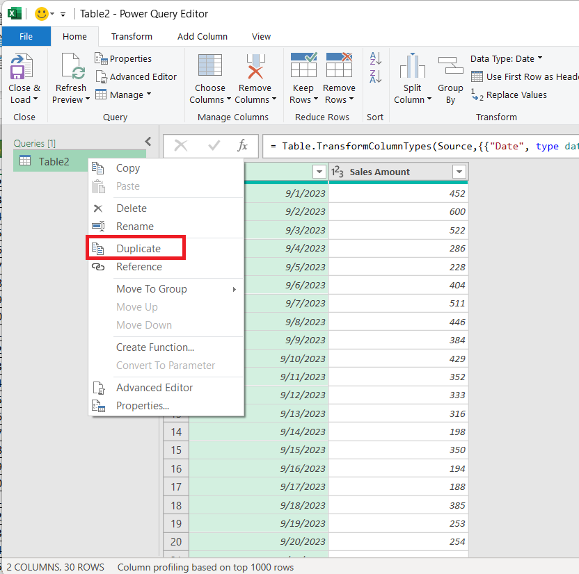
STEP 4: In the left panel, right-click on the table and select Duplicate.
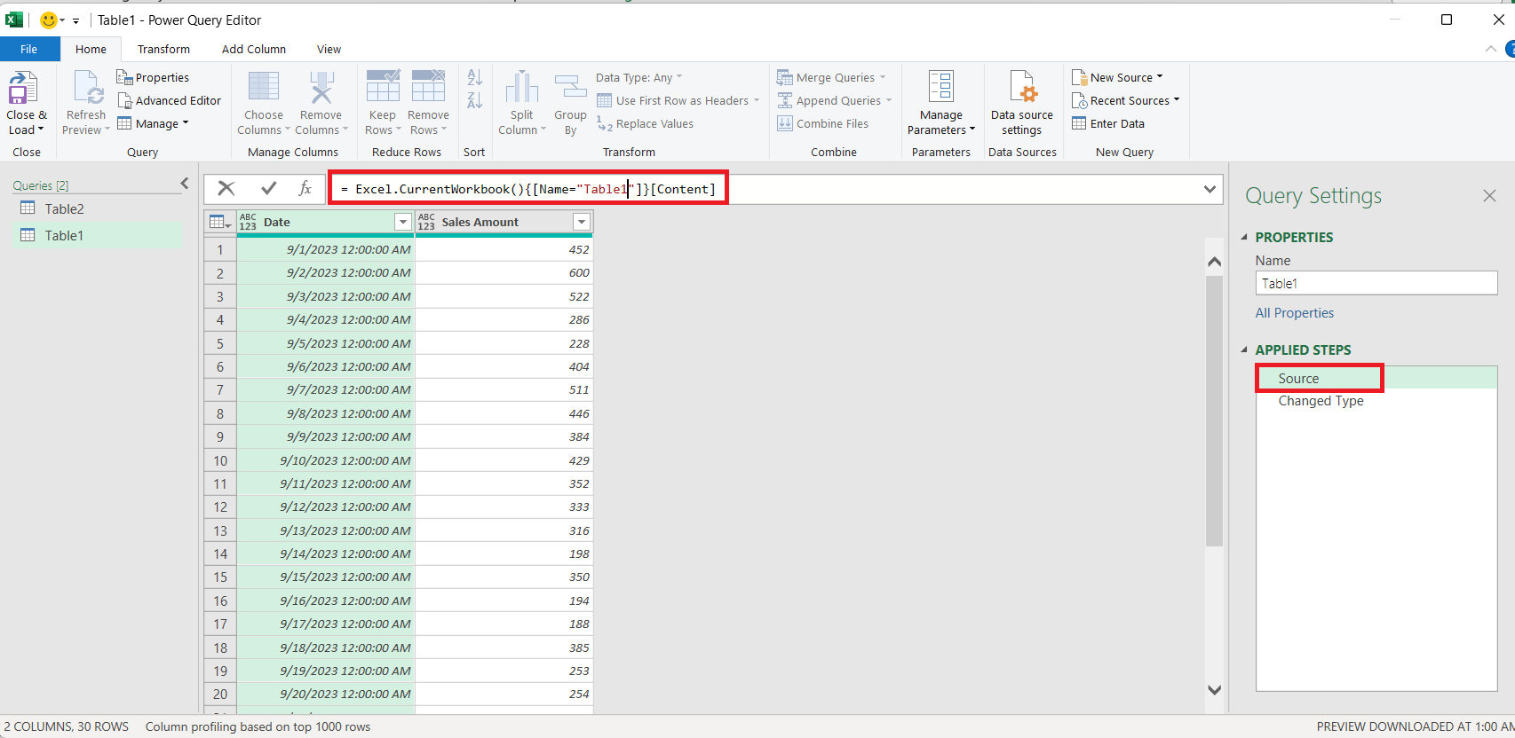
STEP 5: In the Applied Steps section, select Source and edit Table name to Table1.
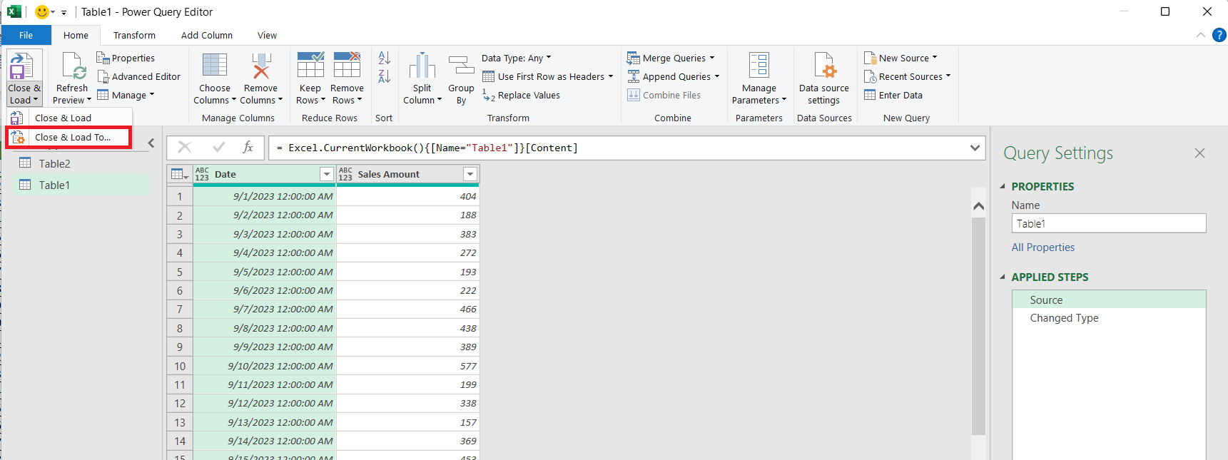
STEP 6: Click on Close & Load > Close & Load To.
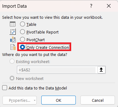
STEP 7: In the Import Data dialog box, select Only Create Connection. Click OK.
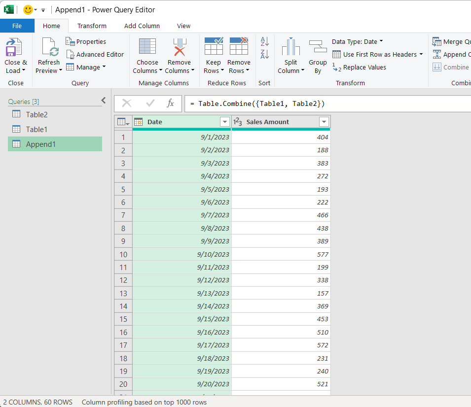
STEP 8: In the Power Query Editor window, go to Append Queries > Append Queries as New.
STEP 9: In the Append dialog box, select Table1 as the First Table and Table2 as the Second Table.
A combined data table will appear as a new query.
STEP 10: Click on Close & Load.
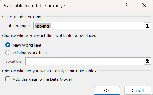
STEP 11: Click on Insert > PivotTable. In the dialog box, select OK.
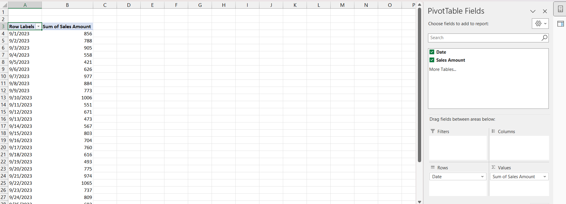
A Pivot Table will be created with the combined data from both regions – East and West.
Conclusion
Pivot tables are invaluable tools for data analysis, especially when dealing with large and complex datasets. It provides a dynamic and user-friendly way to explore and present data and make tasks much more manageable.
However, a common challenge people encounter when working with Pivot Tables is the uncertainty surrounding how to present data across multiple sheets. This article will help you in dealing with the same. By following the steps outlined in this article, you can consolidate data from multiple sheets, establish relationships between them, and build insightful pivot tables.
Further learning:
- Refresh External Data Source in Excel Pivot Table
- Change Data Source in Pivot Table
- Change Count to Sum in Excel Pivot Tables
Click here to access Microsoft’s tutorial on Creating PivotTable from Multiple Sheets in Excel!
John Michaloudis is a former accountant and finance analyst at General Electric, a Microsoft MVP since 2020, an Amazon #1 bestselling author of 4 Microsoft Excel books and teacher of Microsoft Excel & Office over at his flagship Academy Online Course.
