Customising Excel Pivot Table Styles

What if even with this multitude of predefined options, you still want to make your own style? You can easily do that by customising pivot table styles. There are a couple of ways to do this!

Exercise Workbook:

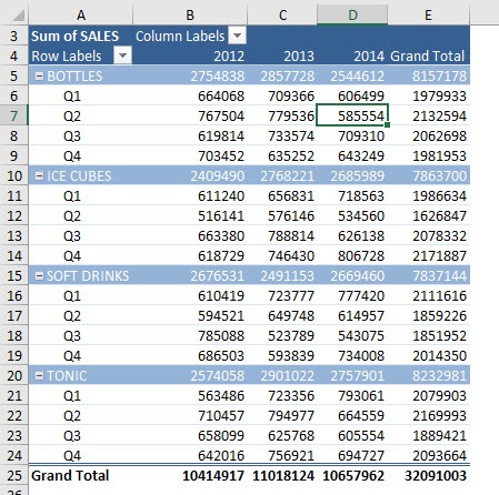
Here is our Pivot Table:

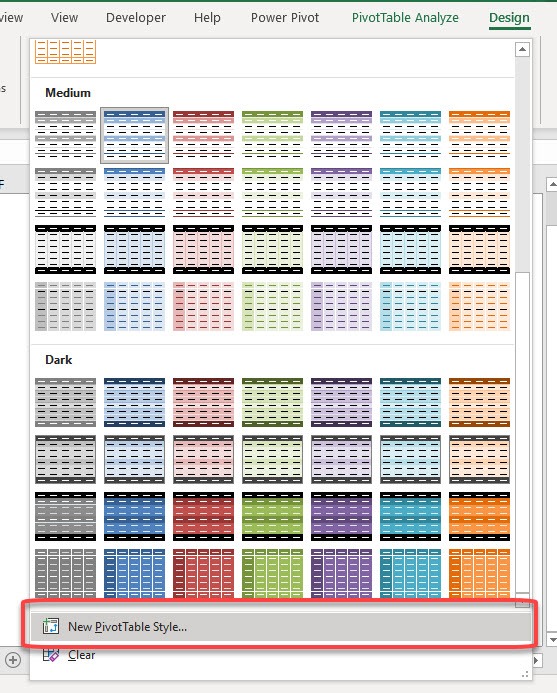
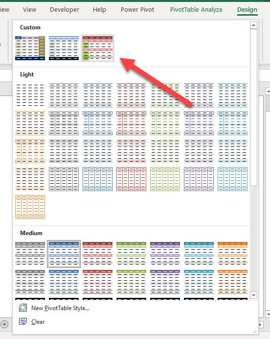
STEP 1: Go to Design > PivotTable Styles and click the down arrow to open the options

If you want to create a new custom style from scratch, select New PivotTable Style

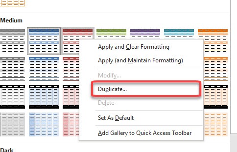
STEP 2: If you have a starting point in mind, you can right-click on any style and select Duplicate

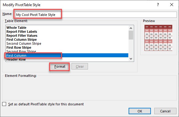
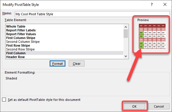
STEP 3: Change the Name into your own preference. There are a lot of elements you can format!

For our example, let us try out First Column. Select that and click Format.

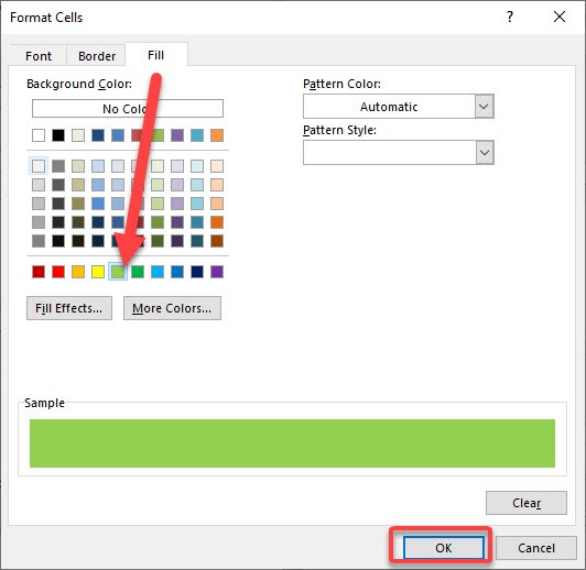
STEP 4: Try out any formatting that you want. We can try out to change the Fill color. Click OK

STEP 5: You can see a preview of how it looks like. Our first column did change its fill color! Click OK

STEP 6: The new style that we created is not applied yet automatically.

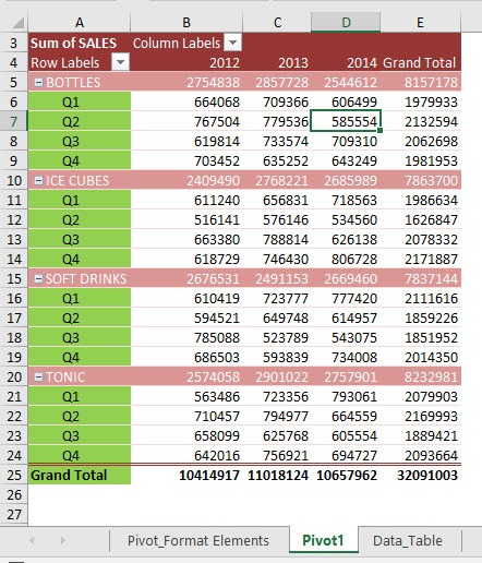
To use that, go to Design > PivotTable Styles and select the new style that we have created

And there you have it!

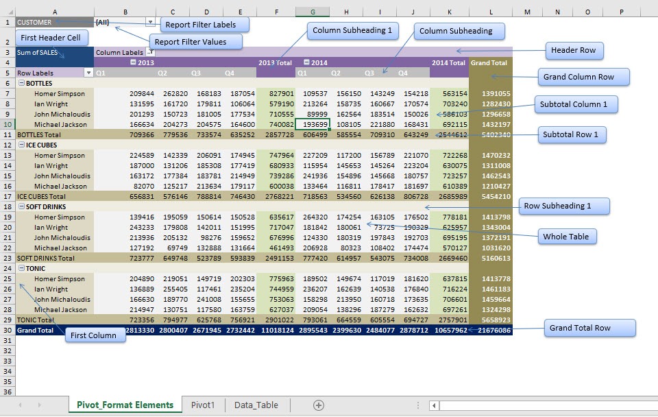
I have also created this diagram for you to immediately see the different Pivot Table Elements. Have fun creating and customising pivot table styles!

Bryan

See also  Filter by Values - Between

Bryan is a best-selling book author of the 101 Excel Series paperback books.