Ever had multiple related tables and wondering how to create a report that connects them together in a single Pivot Table? We have just the thing with Data Model and Relationships!
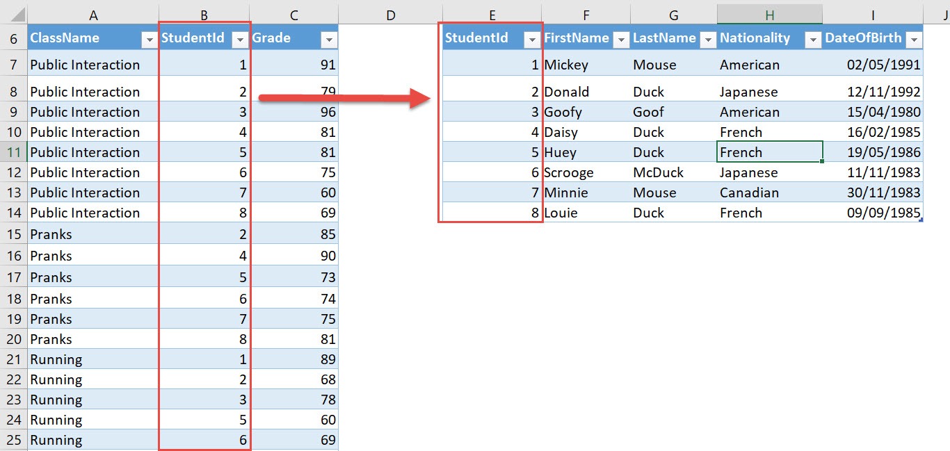
This is our data that we will use. What we want to do is create a report that shows the First Name of the student and the Number of Classes that the student has taken.
The tricky part here is the First Name is in the Students Table, while the number of classes can be retrieved from the Classes Table. Both tables are linked by the StudentId column.
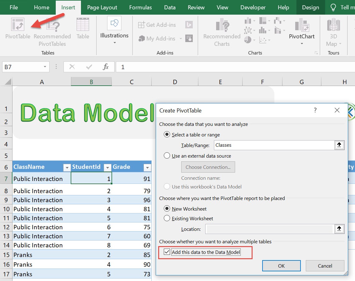
STEP 1: Select the Classes Table. Go to Insert > Pivot Table > New Worksheet
Make sure to tick Add this data to the Data Model. Click OK.
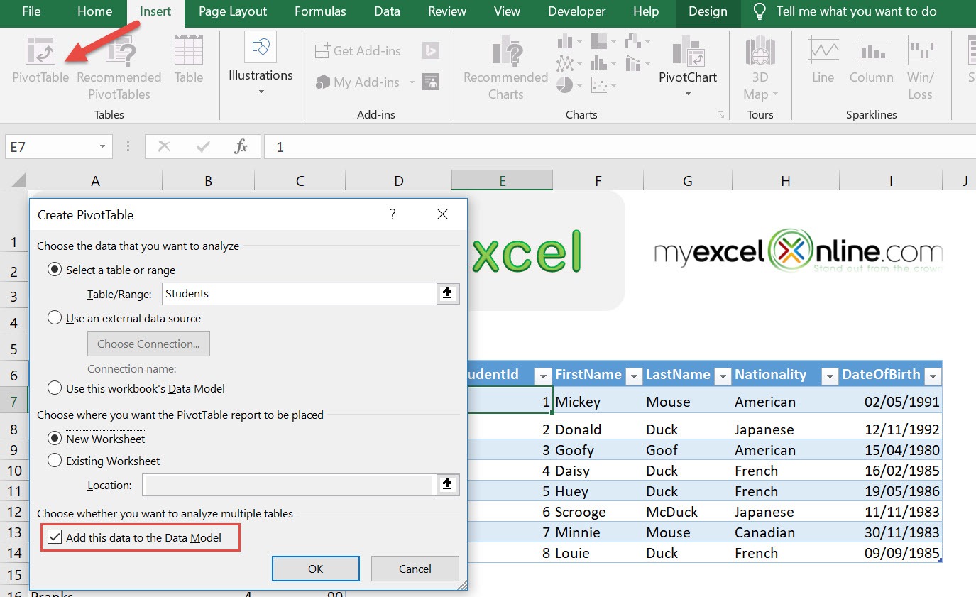
STEP 2: Select the Students Table. Go to Insert > Pivot Table > New Worksheet
Make sure to tick Add this data to the Data Model. Click OK.
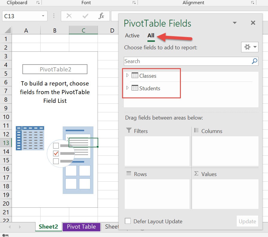
STEP 3: Click All in PivotTable Fields and you should see both tables there.
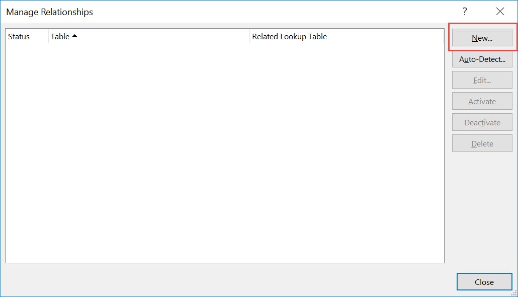
STEP 4: Now we need to link them together! Go to PivotTable Tools > Analyze > Calculations > Relationships
Click New.
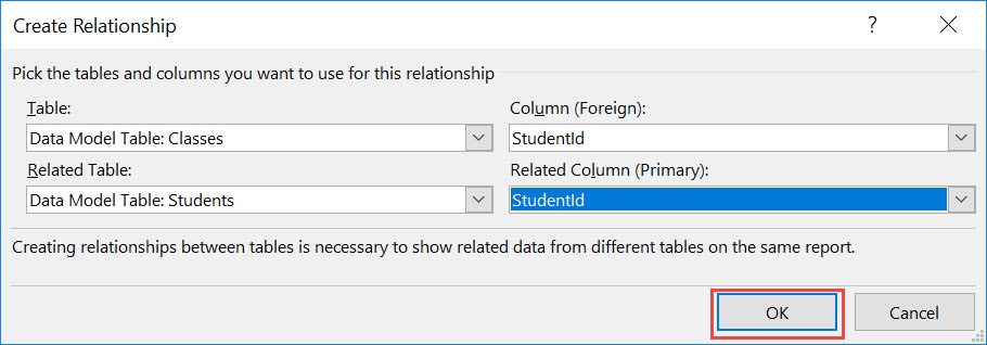
STEP 5: There are 2 sides of a relationship when we want to link them together.
The rule of thumb, is the primary table should have no duplicates. This is the Students table as it does not have duplicate Student Ids.
Set the following then Click OK.
Table – Classes
Column – StudentId
Related Table – Students
Related Column – StudentId
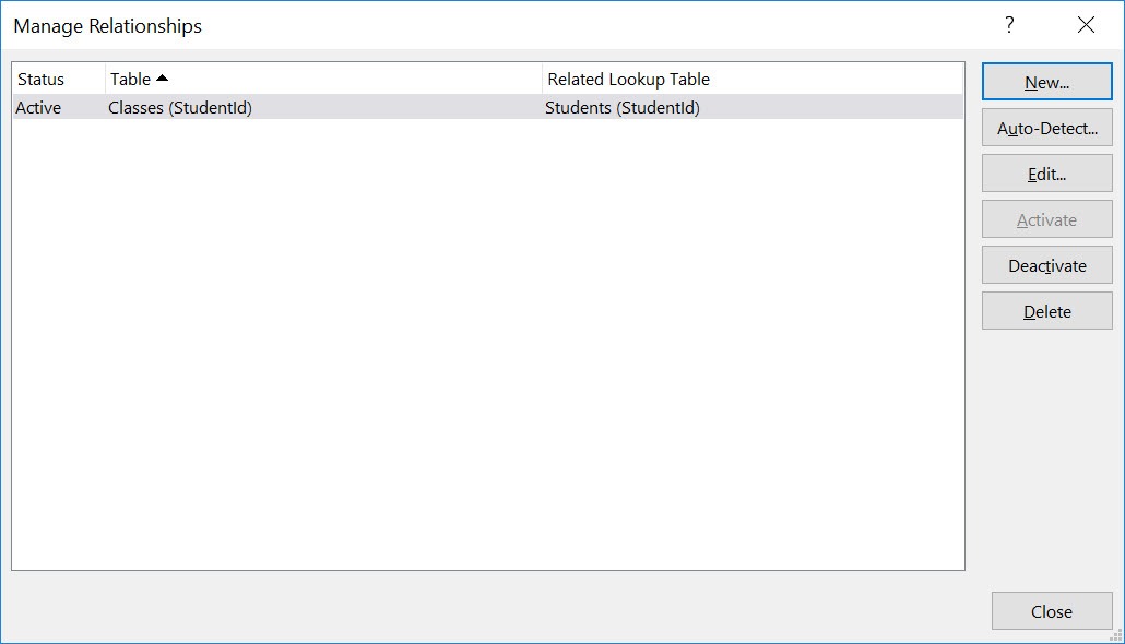
Click Close.
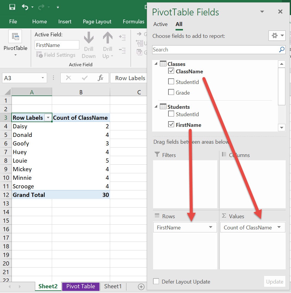
STEP 6: In the ROWS section put in the Students(FirstName) field. In the VALUES section put in the Classes (ClassName) field.
With just that, you can see that Excel was able to show the results in a merged fashion! You can see Daisy has 2 classes enrolled. And from the individual tables, you would not have that information readily available!
Further Learning:
- Clean Data Set for Pivot Table
- Prepare Data for Excel Pivot Tables
- Move and Remove Fields and Items in Excel Pivot Tables
Helpful Resource:
Bryan
Bryan is a best-selling book author of the 101 Excel Series paperback books.
