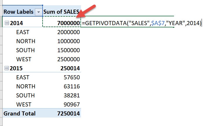
When you wanted to reference a cell in a Pivot Table, a GETPIVOTDATA formula shows up instead. If you want to have just a normal cell reference show up, you can disable/enable get pivot data using Excel Macros!
Make sure your Excel has the Developer Tab enabled following this tutorial.
I explain how you can do this below step by step!
What does it do?
Disable / Enable Get Pivot Data
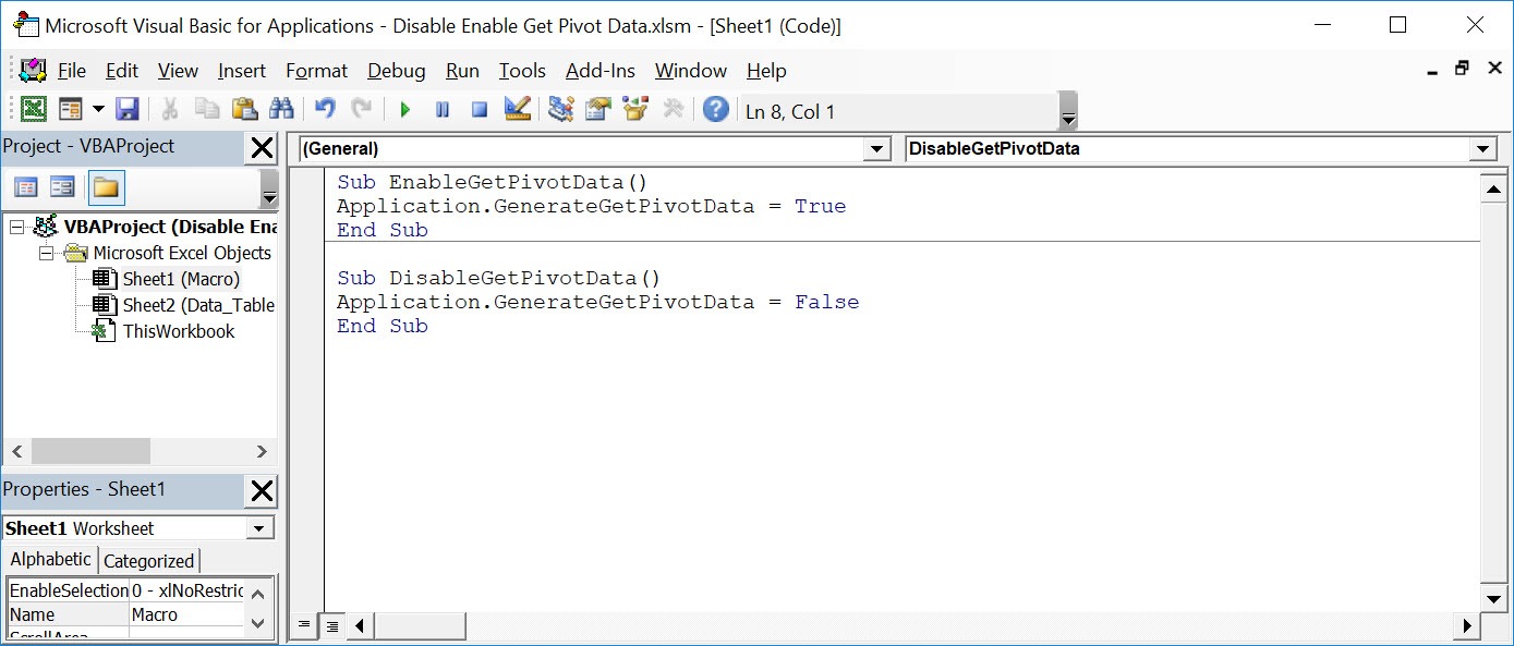
Copy Source Code:
Sub EnableGetPivotData()
Application.GenerateGetPivotData = True
End Sub

Sub DisableGetPivotData()
Application.GenerateGetPivotData = False
End Sub
Final Result:
Exercise Workbook:
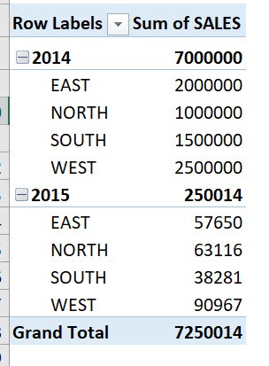
Here is our pivot table:
If we try to create a formula involving one of the cells inside the Pivot Table, you will see the GETPIVOTDATA Formula. Let us change this behavior using Macros!
STEP 1: Go to Developer > Code > Visual Basic
STEP 2: Paste in your code and Select Save. This will create two options for you to choose either to enable or disable. Close the window afterwards.
STEP 3: Let us test it out!
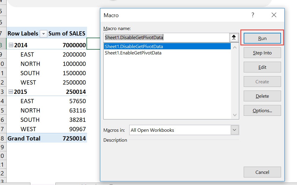
Open the sheet containing the data. Go to Developer > Code > Macros
Make sure your disable macro is selected. Click Run.
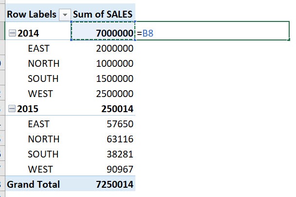
Try referencing a cell inside the pivot table again. It is now a normal cell reference.
With just one click, we have disabled get pivot data!
How to Disable/Enable Get Pivot Data Using Macros In Excel
Bryan
Bryan is a best-selling book author of the 101 Excel Series paperback books.
