Excel 2013 added some new features to its arsenal and one that has been well overdue was the distinct or unique count.
Previously when we created a Pivot Table and dropped a Customers field in the Row Labels and then again in the Values area we got the “total number of transactions” for each customer.
But what about if we want to show the total unique customers?
In Excel 2013 we can, by using the newly created Pivot Table Data Model:
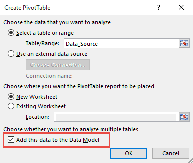
STEP 1: Click in your data source and go to Insert > Pivot Table
STEP 2: The important step here is to “check” the Add this to the Data Model box and press OK
STEP 3: This will create a Pivot Table. Now drop the Customers field in the Row and Values areas which will give you the “total transactions” for each customer
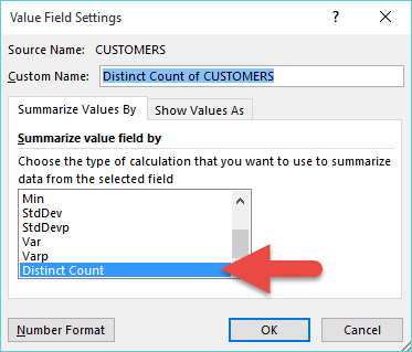
STEP 4: To get a Distinct Count, you need to click on the Values drop down for the Count of Customers and select the Value Field Settings
STEP 5: Under Summarize Values By tab, select the last option, Distinct Count and press OK
See how this is done with the following animated tutorial plus you can download the workbook…
John Michaloudis is a former accountant and finance analyst at General Electric, a Microsoft MVP since 2020, an Amazon #1 bestselling author of 4 Microsoft Excel books and teacher of Microsoft Excel & Office over at his flagship Academy Online Course.


