Microsoft Excel can be used to record expenditures and incomes, create budget plans, forecasts, create data charts, and much more.
I have an Excel secret to share with you!
You can also do Financial Calculations using Excel as a Time Value of Money Calculator.
It can help you in making Excel Finance decisions by incorporating the worth of money in relation to time. It is an extremely useful tool for investment bankers and financial analysts.
When Using Excel as a Time Value of Money Calculator, you will be working on the following financial functions:
- 1 – Present Value (PV)
- 2 – Future Value (FV)
- 3 – Number of Periods (NPER)
- 4 – Interest Rate (RATE)
- 5 -Periodic Payments (PMT)
Let’s look at each of these functions one by one!
1. Present Value (PV)
If you want to know the present value of an investment based on a series of future payments, assuming constant periodic payments and a fixed interest rate, you can use the Excel PV function.
In Excel Finance, future payments can either be periodic constant payments or a lump sum amount at the end of the investment period.
The syntax of the PV Function is:
=PV(rate, nper, pmt, [fv],[type])
What it means:
=FV(interest rate, number of periods, periodic payment, initial amount)
- rate – Interest rate per period
- nper – Total no of compounding periods
- pmt – Annuity amount per period. If this is omitted, make sure you provide Excel with a PV.
- [fv] – Future value of the investment. This is an optional argument.
- [type] – It is should be 0 if the annuity is received at the end of the compounding period and 1 if it received at the beginning of the compounding period. This is an optional argument and by default, its value is set to 0.
To get a better understanding of this function in Excel Finance, let’s look at an example!
Follow the step-by-step tutorial below to understand how to use time calculator Excel and make sure to download the workbook to follow along:
Download excel workbookEXCEL-FINANCIAL-CALCULATOR-1.xlsx
Example 1:
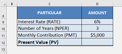
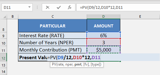
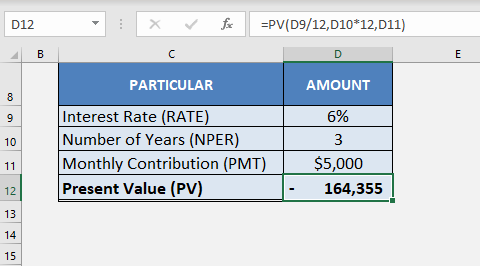
You make an investment of $5,000 each month for a period of 3 years at an interest rate of 6% per annum. Using Excel as a Time Value of Money Calculator, calculate the present value of your investment.
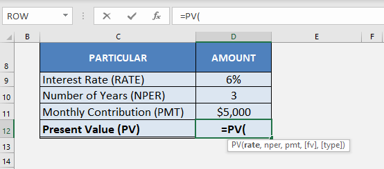
STEP 1: Insert the PV function in cell D12.
=PV(
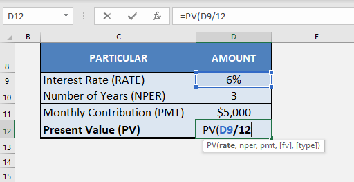
STEP 2: Insert the first argument of the function – RATE (in cell D9)
The periodic payments are paid monthly so the interest rate should also be monthly. Here, you will have to divide the rate by 12 to get the monthly interest rate.
=PV(D9/12,
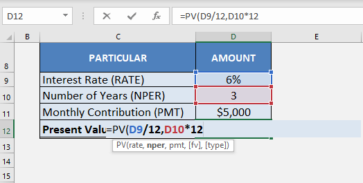
STEP 3: Insert the number of periods mentioned in cell D10.
Each payment is made monthly, so the number of periods will be the number of years multiplied by 12.
=PV(D9/12, D10*12,
STEP 4: Insert the constant payment amount mentioned in the cell D11.
=PV(D9/12, D10*12, D11)
Once you insert the three arguments in the function, Excel will display the present value of the investment.
Make sure to keep the following few points in mind:
- Since monthly payments are made monthly, it is necessary to convert the annual interest rate into a monthly rate.
- The future value calculator is zero and the payments are made at the end of each month, both [fv] and [type] can be omitted here.
- The Present value calculated by Excel is a negative value, as it is an outgoing payment.
To follow the tutorial on the PV function by Microsoft Excel, Click Here.
2. Future Value
Excel’s FV function can be used to determine the future payment for a loan based on the periodic constant payment and a constant interest rate.
The syntax of the FV Function is
=FV(rate, nper, pmt, [pv],[type])
Example 2:
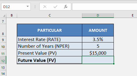
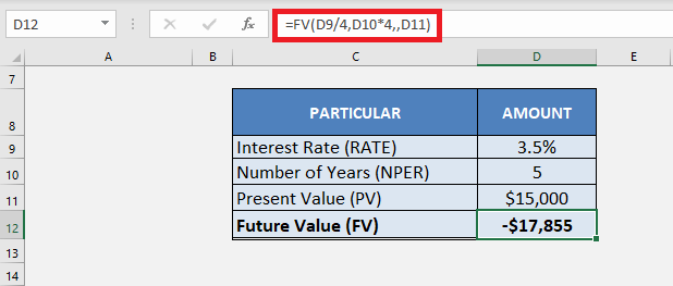
Suppose you have to borrow $15,000 at an interest rate of 3.5% (compounded quarterly) for a period of 5 years. What will be the loan amount you need to pay at the end of 5 years?
This can easily be calculated Using Excel as a Time Value of Money Calculator!
Things to note here are:
- The constant payment amount (PMT) and the type of investment will both be 0.
- The interest rate will be divided by 4 and the number of years will be multiplied by 4 as the interest rate is compounded quarterly.
So, the required formula will be:
=FV(D9/4, D10*4,,D11)
3. Number of Periods (NPER)
Sometimes you know how much you want to invest now and how much you need but you are unsure of the time span. If you know the interest rate you can easily solve for the time period using NPER function.
The syntax of the NPER function is:
=NPER(rate, pmt, pv, [fv],[type])
Example 3:
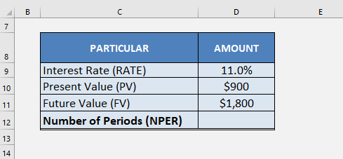
You have $900 to invest today. In how many years will it double if you invest it at an interest rate of 11% compounded annually?
For this example, the present value will be $900 and the future value will be $1800. Since there is no periodic payment, PMT will be 0.
Lastly, you have to change the sign of either PV or FV to negative. It has to done to indicate Excel that one of the amounts is an inflow and the other one is an outflow.
If you skip doing this and leave both PV and FV as positive values, Excel will provide a #NUM error instead of giving you an answer.
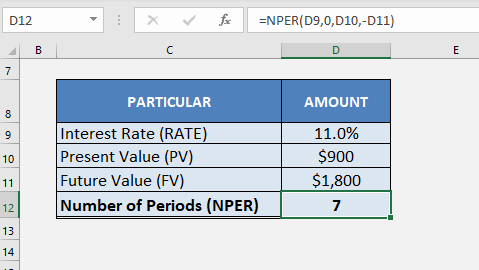
The required formula for Using Excel as a Time Value of Money Calculator will be:
=NPER(D9, 0, D10, -D11)
So, in approximately 7 years your $900 will turn into $1800 if invested at an interest rate of 11% per annum.
4. Interest Rate (RATE)
The RATE function in Excel can be used to find the interest rate for discounting the future value of the investment in present value calculation.
The syntax of the RATE function is :
=RATE (nper, pmt, pv, [fv],[type],[guess])
The last argument of this function is “guess”. It is an optimal argument that is used to provide Excel with an estimate of what the rate could be. If omitted, the default value will be 10%.
Example 4:
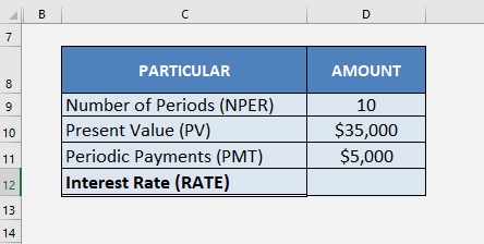
Let’s find out the interest rate on a home loan of $35000 that has to be paid over a period of 30 years with a monthly installment of $5000.
In this example, you can insert the monthly payments made ($5000), the present value of the loan ($35000), and the number of periods (10 years) in the RATE function to get the interest rate.
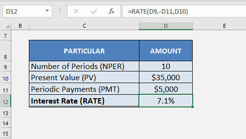
Please note that since the monthly payments are an outflow and the present value of the value received is an inflow, you have to add a negative sign in front of PMT value to get the answer.
The required formula will be:
=RATE (D9, -D11, D10)
This is how you can calculate the loan rate by Using Excel as a Time Value of Money Calculator.
5. PERIOD PAYMENTS (PMT)
The PMT function calculates the periodic payment against an investment or a loan at a constant interest rate for a specified period of time.
The syntax of the PMT function is :
=PMT (rate, nper, pv, [fv],[type])
Example 5:
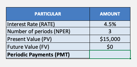
Let’s say you borrowed $15,000 for a period of 3 years. You have to make monthly repayments at the end of each month. What should be the constant monthly payment you should make to repay the entire loan of $15,000 after 3 years?
The payments were made monthly so the interest rate will be divided by 12 and the number of years will be multiplied by 12 to give you the number of periods.
Also, you have to enter both PV and FV in this example so make sure to put a negative sign in front of one of the variables.
Enter FV as 0 as you aim to repay the entire loan amount!
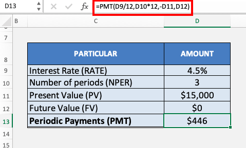
The formula to be used for this calculation is:
=PMT (D9/12, D10*12, -D11,D12)
You have to make a monthly payment of $446 for a period of 3 years to repay the loan amount of $15,000.
Conclusion
By supplying any three of the five variables of a Time Value of Money problem, you can easily get the required answer. This can be done by Using Excel as a Time Value of Money Calculator.
There are many more useful financial functions available in Excel. Click here to learn more about it!
Click here to take a look at the tutorial on Financial Functions by Microsoft.
Further Learning:
- A Comprehensive Guide to Descriptive Statistics in Excel
- Master ANOVA in Excel: A Step-by-Step Tutorial
- Useful Excel Solver Functions for Optimal Data Analysis
John Michaloudis is a former accountant and finance analyst at General Electric, a Microsoft MVP since 2020, an Amazon #1 bestselling author of 4 Microsoft Excel books and teacher of Microsoft Excel & Office over at his flagship Academy Online Course.
