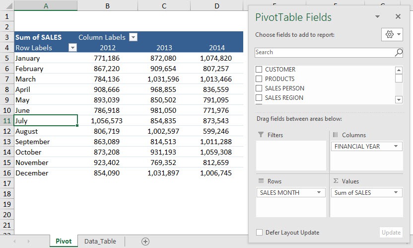
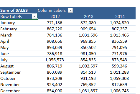
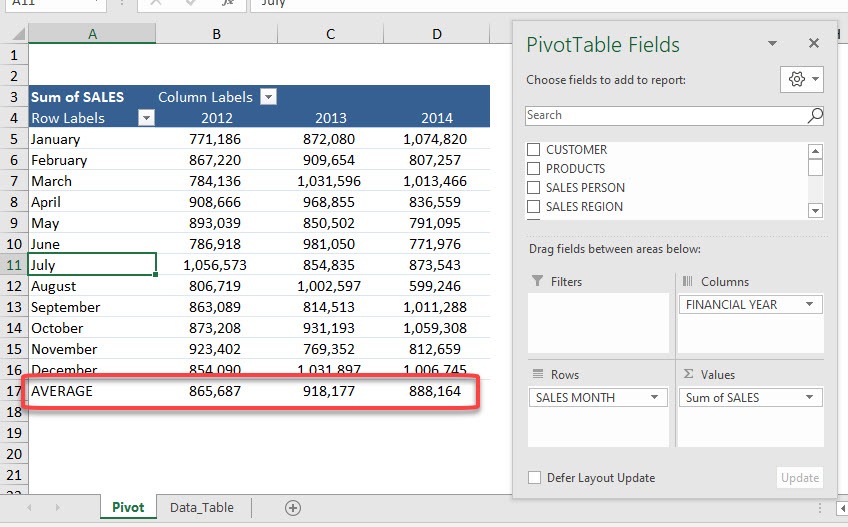
Here is our current Pivot Table setup:
You can easily add another row that calculates the average sales for each year using formulas in calculated items. Let’s see how it can be done!
Download the Excel Workbook below and follow the step-by-step tutorial below to add Excel formulas in Calculated Items.
STEP 1: Click on any cell in the Pivot Table.
This will display PivotTable Analyze and Design tabs.
STEP 2: Go to PivotTable Analyze > Fields, Items & Sets > Calculated Item
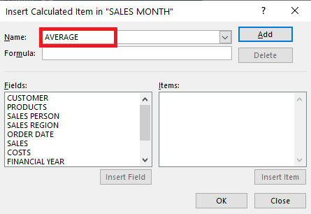
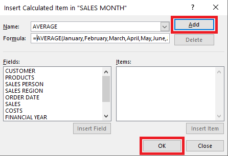
STEP 3: In the Name box, type in a name that you prefer for the formula.
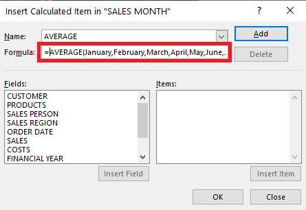
STEP 4: In the Formula box, type in the Average Function:
= AVERAGE(January,February,March,April,May,June,July,August,September,October,November,December)
STEP 5: Click Add then OK
Your Calculated Item is now ready!
Edit Formula in Calculated Item
If you wish to edit the formula from an average of 12 months to an average of 3 months, you can do that as well:
STEP 1: Click on any cell in the Pivot Table.
This will display PivotTable Analyze and Design tabs.
STEP 2: Go to PivotTable Analyze > Fields, Items & Sets > Calculated Item
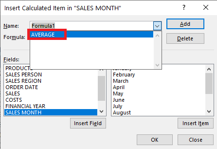
STEP 3: In the Name box, select the formula.
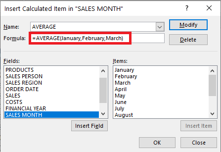
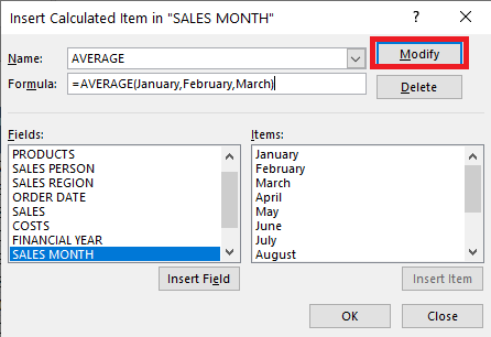
STEP 4: Edit the formula.
= AVERAGE(January,February,March)
STEP 5: Click Modify.
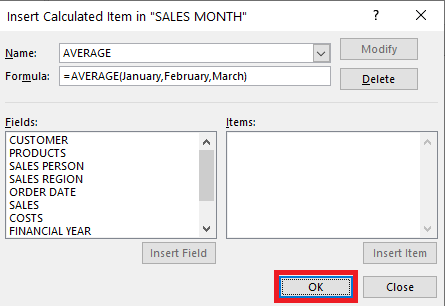
STEP 6: Click OK.
Delete Formula in Calculated Item
You can delete the formula from the Pivot Table calculated item by following the steps below:
STEP 1: Click on any cell in the Pivot Table.
STEP 2: Go to PivotTable Analyze > Fields, Items & Sets > Calculated Item
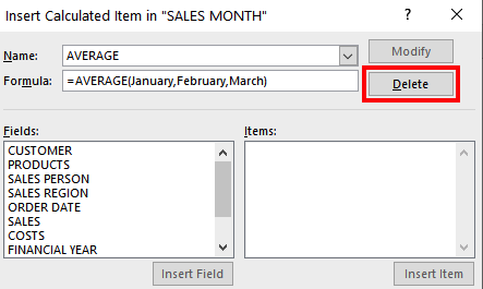
STEP 3: In the Name box, select the formula.
STEP 4: Click Delete.
This is how you can easily create formulas in a calculated item, edit them or even delete them if it is not required anymore.
Click here to learn more about Pivot Table Calculated items!
Make sure to download our FREE PDF on the 333 Excel keyboard Shortcuts here:
Bryan
Bryan is a best-selling book author of the 101 Excel Series paperback books.
