Excel´s hyperlink capability is amazing but many people don’t use it as they don’t know its full capabilities.
With a hyperlink you can link an object/text to open an existing file on your desktop, go to a website, open up an email to a specific contact or go to a cell within your workbook.
I will show you in the example below how you can create a hyperlink in a shape and then click on the shape to go to a specific report within your workbook without the need to scroll.
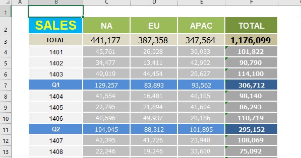
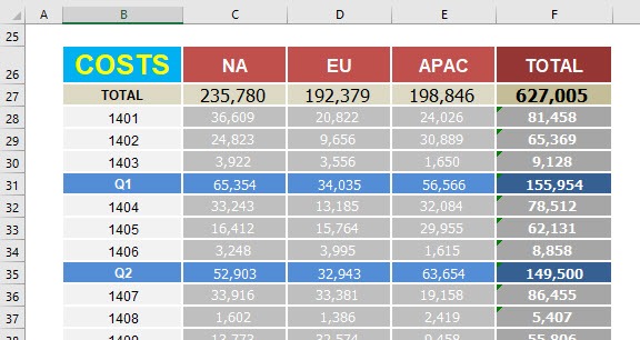
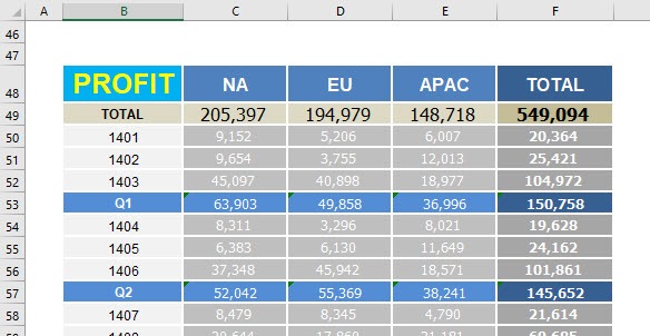
To have a better idea, this is how our workbook is setup, we have 3 main sections that we want the buttons to navigate to:
1. Sales
2. Costs
3. Profit
Download workbookHyperlink-Buttons1.xlsx
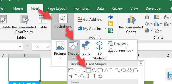
STEP 1: Go to Insert > Illustrations > Shapes > Any Rectangle Shape
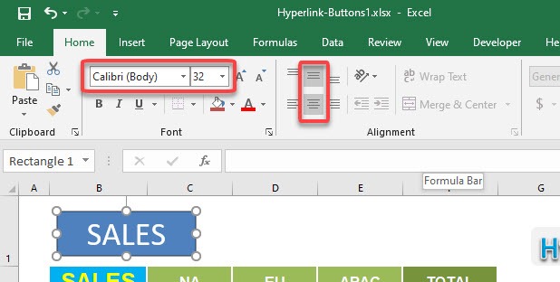
STEP 2: Create a rectangle and type SALES. Update the formatting to make the text look bigger and centered.
STEP 3: While holding CTRL + SHIFT, drag your first button using left-click to instantly duplicate it. Do it twice.
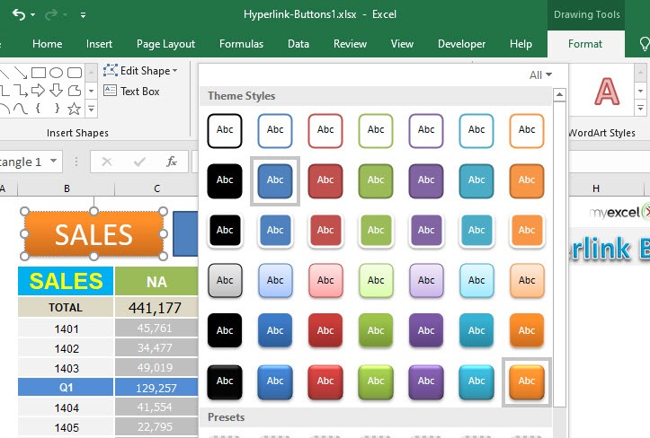
STEP 4: Go to Format > Shape Style and pick the formatting you want. Do it for all buttons to differentiate them from one another.
Make sure to change the text of the other buttons to COSTS and PROFIT.
STEP 5: We will now create the cell that our button will navigate to.
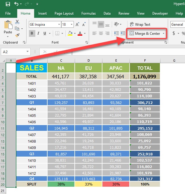
Select the blank cells beside the SALES table. Then select Home > Merge & Center
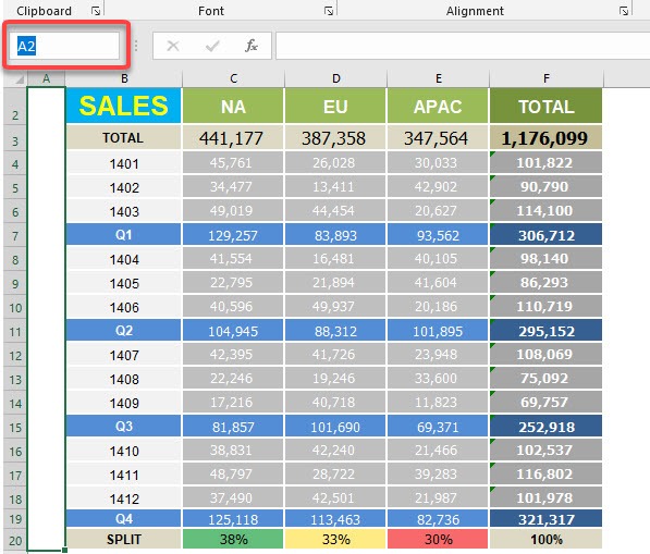
STEP 6: Take note of the cell reference and copy this. For SALES this is cell A2.
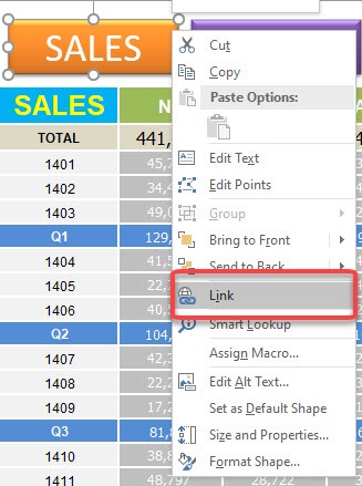
STEP 7: Right click on the SALES Button and select Link.
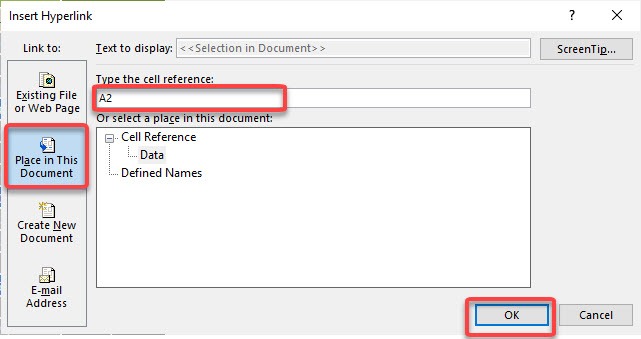
STEP 8: Make sure Place in This Document is selected then place the cell reference A2. Press OK.
STEP 9: Do the same for COSTS.
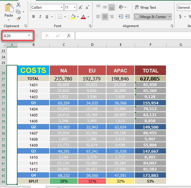
Select the blank cells beside the COSTS table. Then select Home > Merge & Center
Take note of the cell reference and copy this. For COSTS this is cell A26.
STEP 10: Right click on the COSTS Button and select Link.
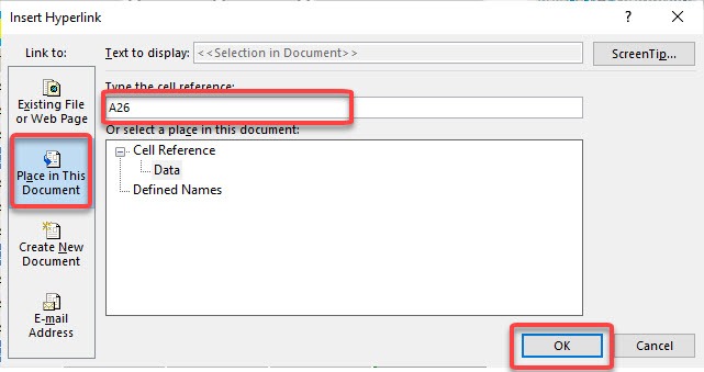
Make sure Place in This Document is selected then place the cell reference A26. Press OK.
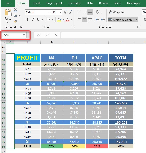
STEP 11: Select the blank cells beside the PROFIT table. Then select Home > Merge & Center
Take note of the cell reference and copy this. For PROFIT this is cell A48.
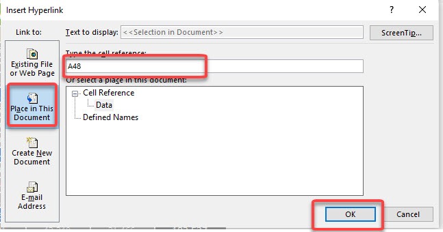
STEP 12: Right click on the PROFIT Button and select Link.
Make sure Place in This Document is selected then place the cell reference A48. Press OK.
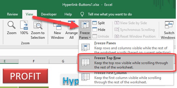
STEP 13: Let’s freeze in place the top row that contains our buttons.
Go to View > Freeze Panes > Freeze Top Row
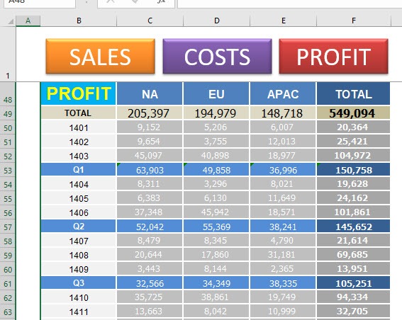
Now try clicking on the buttons and you will be impressed with the instant navigation!
John Michaloudis is a former accountant and finance analyst at General Electric, a Microsoft MVP since 2020, an Amazon #1 bestselling author of 4 Microsoft Excel books and teacher of Microsoft Excel & Office over at his flagship Academy Online Course.
