Excel Indirect function can be used to return a valid reference from a given text string.
The cell reference provided in this formula will not change when you add or delete rows and/or columns. For Example, =INDIRECT(A1: E1) will always refer to the first 5 columns of the sheet even if new columns are added or deleted.
In this article, you will learn in details regarding the following:
- Excel Indirect Function
- Basic use of Indirect Function
- Reference A Cell in Another Sheet
- Reference a Range of Cells in Another Sheet
- Conclusion
Excel Indirect Function
This function does not perform any calculation or evaluate any logic or condition.
So, What does it do?
Excel Indirect function is used to indirectly reference a cell, or a range of cells of a sheet.
Formula breakdown:
=INDIRECT(ref_text, [a1])
What it means:
ref_text – return the referenced range
[a1] – specify the type of reference (A1 style or R1c1 style) mentioned in ref_text. Omit or type TRUE if the reference is an A1 style or enter FALSE if it is an R1C1 style.
The type of references are:
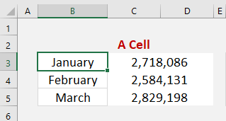
- A1 style – This is the most common reference that we use when we are trying to provide cell reference. In this, you first provide the column number (indicated by A, B, C, etc) and then the row number (indicated by 1, 2, 3, etc). Example, the highlighted cell in the image below is B3
- R1C1 style – This reference is opposite to the A1 style i.e. first the row number and then column number. For example, R3C2 refers to cell B3 which is row 3 and column 2 in a sheet.
The INDIRECT function is really cool as it can be used to reference sheet cells or a range of cells.
It opens up a lot of interesting possibilities as you can have fun creating flexible formulas, like indirectly summing the values that reside in another worksheet!
Let’s look at a basic example to understand how this function works!
Basic use of Indirect Function
In the example below, you have used the Indirect function to return a value when the referenced range is a cell.
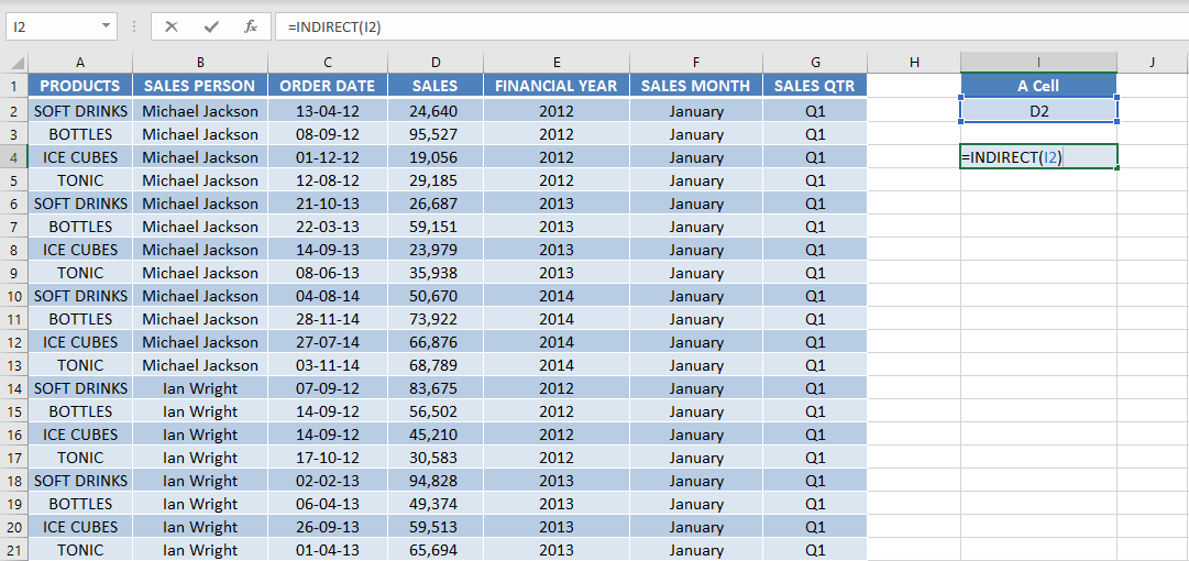
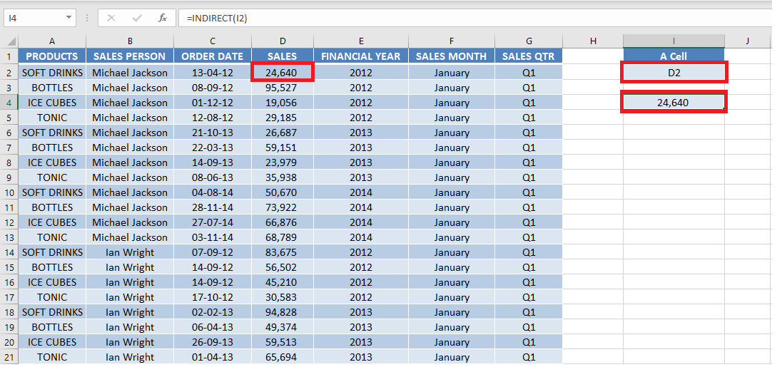
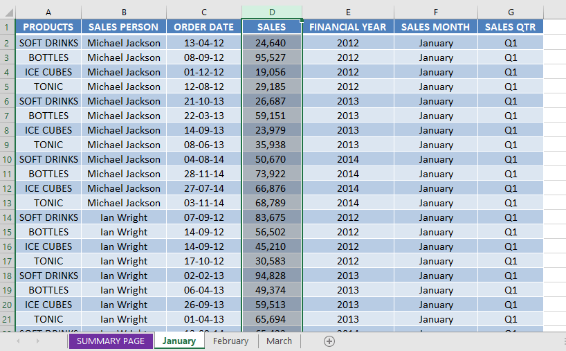
You have the sales amount 24,640 stored in cell D2 and the text D2 stored in cell I2.
Now, when you type the formula =INDIRECT(I2) Excel will follow the steps below:
- It will first go to cell I2 which the formula refers to and get the value D2.
- Next, it will go to cell D2 and pick the value 24,640 and display that result.
As you can see, the Excel Indirect Function converts the text string D2 into a cell reference.
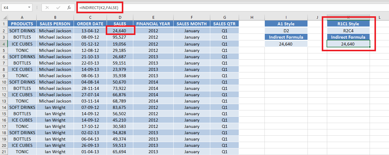
Using R1c1 style, the same formula will be: =INDIRECT(K2, FALSE)
Cell K2 contains the cell reference in the R1C1 style.
Make sure to provide the second argument of the function i.e. [a1]. Here, it is FALSE.
Until now, you have covered how to use Excel Indirect function when you are trying to fetch values from the same sheet.
Let’s see how it works when you want to use an Excel reference cell in another sheet dynamically!
Reference a Cell in Another Sheet
When the referenced range is a cell of a Sheet, the Excel INDIRECT function will go and return the content of the referenced cell in that Sheet.
Read below to learn how to insert Sheet reference in Excel Indirect Formula.
Watch it on YouTube and give it a thumbs-up!
Make sure to download the Excel Workbook below and follow along:
Download excel workbookIndirect-Sheet-Reference.xlsx
In this example, you have two Excel Indirect Sheet name – Summary Page & January.
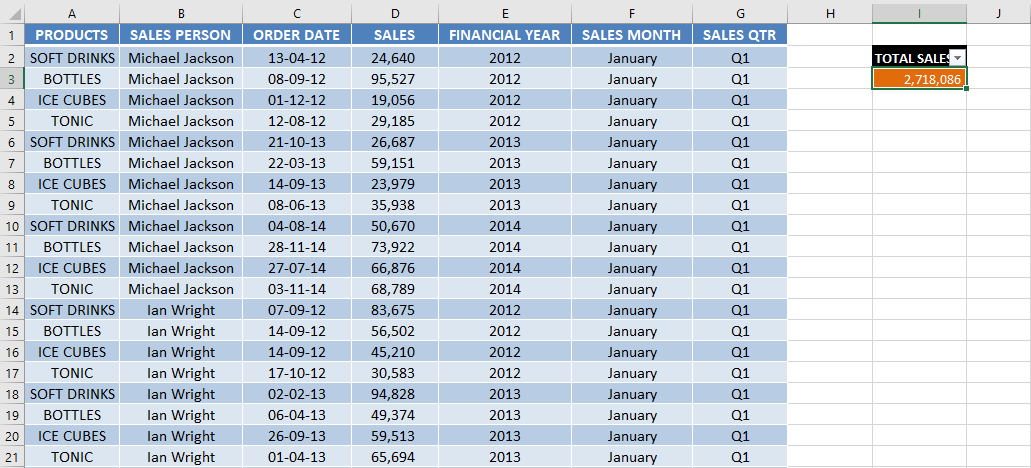
In Sheet – January, you have sales data for the month of January and a total sales amount achieved in that month mentioned in cell I3.
In the sheet – Summary Page, you want to pull the total sale figure in cell E11.
You can use the formula below:
=INDIRECT(“JANUARY!I3”)
Sheet references are in the format of SHEETNAME!CELL, an example would be January!I3 which would mean the cell I3 in the worksheet named January.
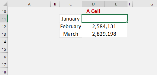
Say we enter in cell C11 the worksheet name: January
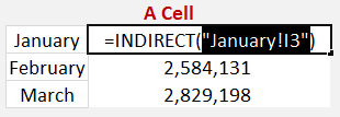
In another cell, we enter =INDIRECT(C11&”!I3″), which will translate into =INDIRECT(“January!I3”) as the ampersand & will concatenate/join the two strings together.
NB: Highlighting the contents between the parenthesis and pressing the F9 key will confirm this:
This will indirectly return the value that resides in cell I3 in the worksheet named January, which has the total sales amount of $2,718,086 in our example below:
This is how Excel sum indirect another sheet reference works!
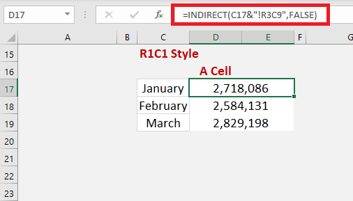
The same formula for R1C1 style will be: =INDIRECT(C17&”!R3C9″,FALSE)
Reference a Range of Cells in Another Sheet
When the referenced range is a range of cells of a Sheet, the Excel INDIRECT function will go and return the content of the referenced cells of that Sheet.
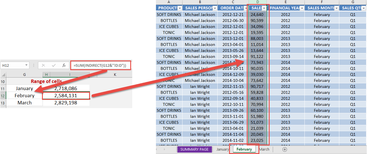
Instead of fetching the summation value from one cell, you can pull data from a range of cells i.e. D:D.
You can use the formula below:
=SUM(INDIRECT(“FEBRUARY!D:D”))
We can then enter a SUM function which will total the referenced cells of that sheet.
Say we enter in cell G12 the worksheet name: February
In another cell we enter =SUM(INDIRECT(G12&”!D:D”)), which will translate into =SUM(INDIRECT(“February!D:D”)) as the ampersand & will concatenate/join the two strings together.
This will indirectly Sum the values that reside in column D in the worksheet named February, which is $2,584,131 in the example below (click to expand image):
This is how Excel will use indirect function excel different sheet reference and fetch values from there!
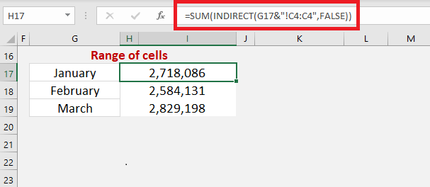
The same formula for R1C1 style will be: =SUM(INDIRECT(G17&”!C4:C4″,FALSE))
Conclusion
In this article, you have learned about Indirect Function in Excel – Syntax, Basic Example, using cell reference A1 style & R1C1 style, when reference cell is in another sheet & when reference is a range of cells in another sheet.
There is a lot that this incredible function – INDIRECT can do. Click here to know all about it!
Further Learning:
- INDIRECT Function for Dependent Dropdown Lists in Excel
- INDIRECT Function in Excel
- How to Master Excel Formulas – The Ultimate Guide
You can learn more about how to use Excel by viewing our FREE Excel webinar training on Formulas, Pivot Tables, and Macros & VBA!
Bryan
Bryan is a best-selling book author of the 101 Excel Series paperback books.
