What does it do?
Searches for a value in the first column of a table array and returns a value in the same row from another column (to the right) in the table array.
Formula breakdown:
=VLOOKUP(lookup_value, table_array, col_index_num, [range_lookup])
What it means:
=VLOOKUP(this value, in this Named Range, and get me value in this column, Exact Match/FALSE/0])
A Named Range makes it easier to understand Excel formulas, especially if the said formula contains an array argument.
A Named Range can be a cell, a cell range, a Table, a function, or a constant.
Watch this video on YouTube to learn more about Vlookup Range:

Follow the step-by-step tutorial on how to use Vlookup with named range and make sure to download the workbook and follow along:
STEP 1: To define a Named Range in Excel you need to select the cell/cell range/Table/function/constant and go to the Name Box which is located on the top left-hand corner of the workbook – next to the Formula Bar.
STEP 2: In here you can name your range whatever you like (make sure there are no spaces) and press Enter. You can view your Named Range by clicking on the drop-down box in the Name Box. In our example, we will give this a name of StockList.
You can also view/edit/delete your Named Range by going to the Formulas tab in the Ribbon menu and selecting Name Manager.
STEP 3: Now that you are all set, each time you are creating a formula, like a Vlookup formula, it is best to use a Named Range as it makes the formula easier to understand and maintain.
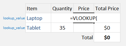
We need to enter the Vlookup function:
=VLOOKUP(
The Vlookup arguments:
Table of Contents
lookup_value
What are we looking for?
Reference the cell that contains the text or value:
=VLOOKUP(G15,
table_array
From which list are we doing a lookup on?
The formula for Excel VlookUp Named Range will be:
=VLOOKUP(G15, StockList,
col_index_num
From which column do we want to retrieve the value?
We want to retrieve the Price which is the SECOND column from our table array:
=VLOOKUP(G15, StockList, 2,
[range_lookup]
Do we want an exact match?
Place in FALSE to signify that we want an exact match:
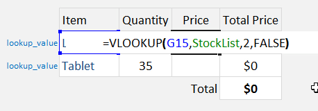
=VLOOKUP(G15, StockList, 2, FALSE)
This is how the price will now dynamically change based on your selection with Vlookup using named range:
Further Learning:
- XLOOKUP vs VLOOKUP: Top 5 Comparison of Excel Lookup Functions
- Why VLOOKUP not working in Excel – Top 5 Problems with Solutions
- 2 Easy Methods on How to Use XLOOKUP with Multiple Criteria
John Michaloudis is a former accountant and finance analyst at General Electric, a Microsoft MVP since 2020, an Amazon #1 bestselling author of 4 Microsoft Excel books and teacher of Microsoft Excel & Office over at his flagship Academy Online Course.


