Mastering the art to extract words from cells in Microsoft Excel is a game-changer for anyone working with extensive datasets. Whether you’re isolating usernames, pulling out domain names, or splitting addresses, understanding how to efficiently use Excel’s substring functions can significantly boost your productivity.
This guide explores the various techniques from basic methods like the LEFT, RIGHT, and MID functions to more complex strategies involving FIND, SEARCH, ensuring you’re equipped to tackle any text manipulation task.
Key Takeaways:
- Begin with the basics by getting comfortable with the LEFT, RIGHT, and MID functions for most straightforward text extraction needs.
- Utilize Excel’s Text to Columns feature for quick and easy splitting of data without the need for complex formulas, perfect for one-off tasks.
- Master nesting functions such as combining LEFT with FIND for extracting names, or MID with SEARCH for domain names, to handle more intricate scenarios.
- Employ TRIM, CLEAN, and SUBSTITUTE functions together for thorough data cleaning, ensuring your datasets are free from excess spaces, non-printable characters, and unwanted text.
Table of Contents
Introduction to Extracting Words in Excel
Overview of Substring Extraction Techniques
When you are dealing with extensive datasets, knowing how to swiftly extract specific information can save you a substantial amount of time. Substring extraction techniques in Excel are designed to do just that – they allow you to pull out bits and pieces of data from larger text entries with precision.
There are multiple ways to tackle substrings in Excel, each with its unique application. You may find yourself using the LEFT, RIGHT, and MID functions for straightforward tasks, while the FIND and SEARCH functions can help you identify positions of specific characters before slicing the string.
For those needing to work with more advanced cases, combining these functions or using them alongside TEXTAFTER and TEXTBEFORE can unlock even more capabilities. Whether you’re working with usernames, domain names, addresses, or other alphanumeric strings, mastering these techniques will significantly enhance your data processing prowess.
Basic Methods to Extract Words from Cell
Getting Started with LEFT, RIGHT, and MID Functions
Embarking on your journey to extract text from cells in Excel? Begin with the foundational trio of substring functions: LEFT, RIGHT, and MID. These are your go-to tools for most basic text manipulation tasks.
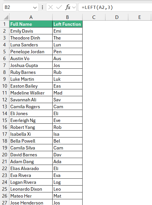
- LEFT Function: Need the beginning part of a string? Use LEFT to pluck out characters from the start of your text. Imagine you havefull names, and you want just the the first three characters; =LEFT(A2, 3) is your friend here.
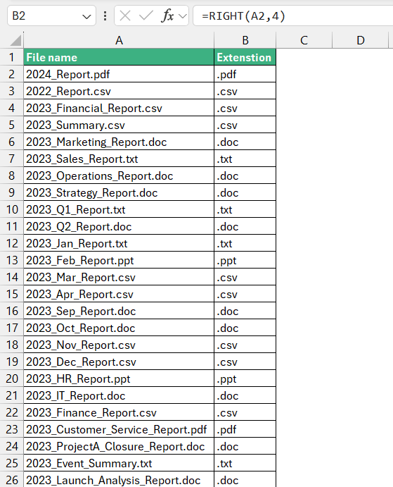
- RIGHT Function: What about the end of a string? That’s where RIGHT comes into play. For instance, if a cell contains file name, and you’re interested in extracting just the extension, =RIGHT(A2, 4) does the job by snatching the last four characters.
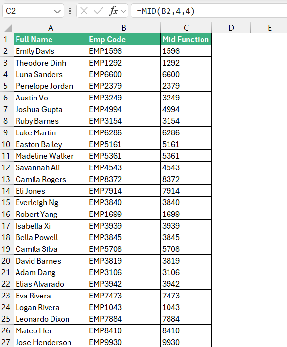
- MID Function: Sometimes, the gold lies in the middle. MID lets you fetch text from any part of the string, beginning at the spot you specify. You’ll need to inform Excel of the starting point and how many characters to retrieve after it. So, to get four characters starting from the fourth position, you’d use =MID(B2, 4, 4).
Remember, these functions become even more powerful when you pair them with SEARCH to locate the position of a character or a substring dynamically, making your formulas adapt to the data they are dealing with.
Text to Columns – A Simple Way to Split Data
For times when you need a break from crafting formulas, Excel’s Text to Columns wizard springs to the rescue! It’s a robust tool for quickly splitting text into multiple cells based on a chosen delimiter, all without the fuss of functions.
Here’s how to put it to use:
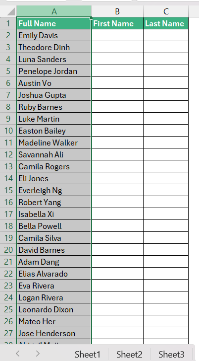
STEP 1: Select the column containing the names or text you wish to dissect.
STEP 2: Navigate to Data > Text to Columns on the ribbon.
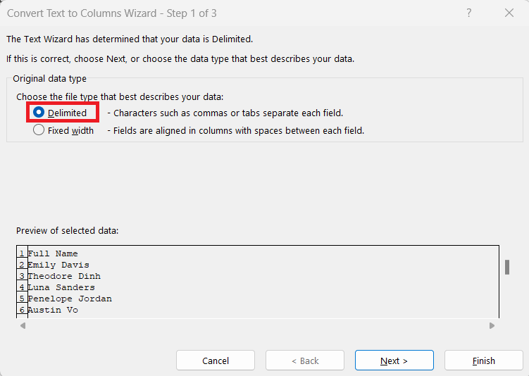
STEP 3: Select Delimited and then click Next.
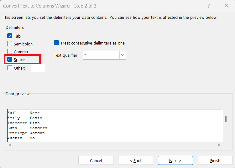
STEP 4: Choose your delimiter, such as a space, comma, or other characters and click Next.
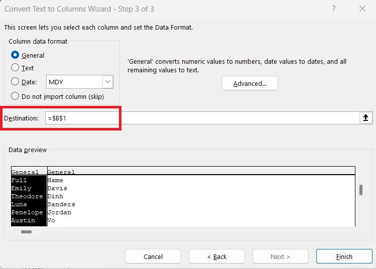
STEP 5: Select the destination cell and click Finish, and voilà!
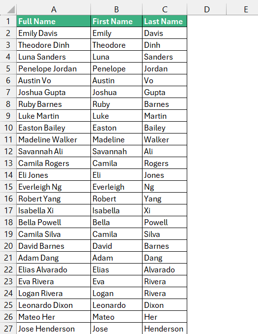
Your text now resides neatly in separate columns.
What sets Text to Columns apart is its simplicity and immediacy, making it perfect for one-off tasks where functions might be overkill. However, for dynamic data updates, you’ll want to stick with functions that adjust automatically.
It’s worth noting that should you need to split data at each occurrence of a specific character repeatedly, Text to Columns might need to be run multiple times. You might also lose the original data in the process if you don’t specify a different destination. Keep these limitations in mind as you choose the best tool for your task.
Real-world Examples of Substring Extractions
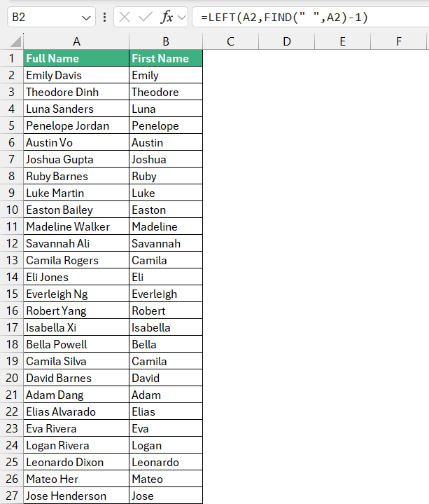
Extracting First Name
Navigating through Excel’s nested functions is like putting together pieces of a puzzle. Each function is a building block, and when they are stacked together, they create sophisticated formulas that can solve intricate problems.
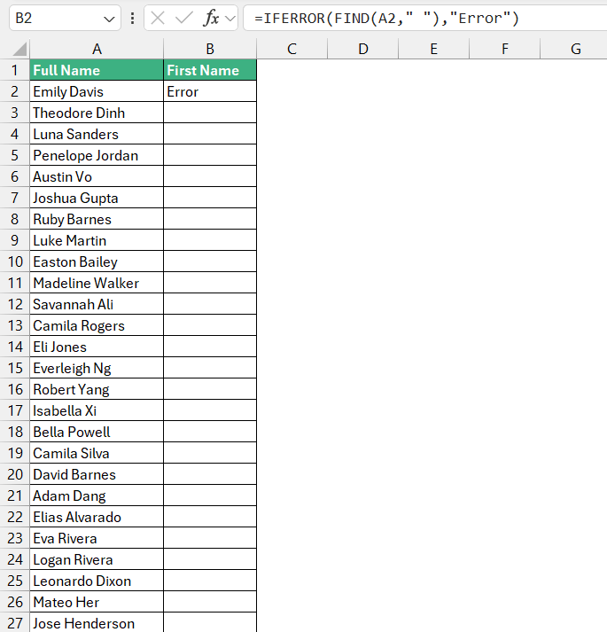
Let’s tackle the concept of nesting—this is when you place one function inside another. For instance, combining LEFT and FIND allows you to cut out a first name from a full name in a cell. The process looks something like this: =LEFT(cell_reference,FIND(" ",cell_reference)-1). Here, FIND determines where the space character is, acting as an argument for LEFT that specifies how many characters to extract.
With practice, these nested marvels will become second nature, expanding your capacity to wrangle data with agility and impact your overall analytical capacity.
Usernames from Email Addresses
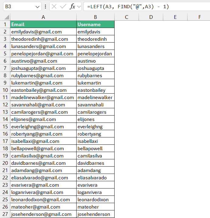
Extracting usernames from email addresses is a common task that illustrates the practical application of Excel’s text functions. It’s a scenario you’re likely to encounter whether you’re managing contact lists, organizing user data, or simply cleaning up a dataset.
To achieve this, the combination of LEFT and FIND functions are typically used. Here’s the formula:
=LEFT(email_cell, FIND("@", email_cell) - 1)
This simple yet effective formula will swiftly isolate usernames, allowing you to manipulate them independently from their domains. Keep in mind that while the username typically precedes the “@”, different email formats and extra characters can complicate the process.
While there are more advanced methods and specialized tools for cleaning and working with email data, mastering this fundamental technique will bolster your Excel toolkit, ensuring that you’re ready to address such challenges with confidence and ease.
This capability to dissect crucial components of data extends beyond just emails, showcasing why Excel remains a powerful ally in anyone’s data analysis arsenal.
Domain Names and Street Addresses: More Than Just Text
When handling domain names and street addresses, you’re dealing with more than mere text strings – you’re facing structured data with its own rules and complexities. Domain names, for instance, have specific segments like top-level domains (.com, .org), while street addresses come with numbers, names, directions, and possibly more.
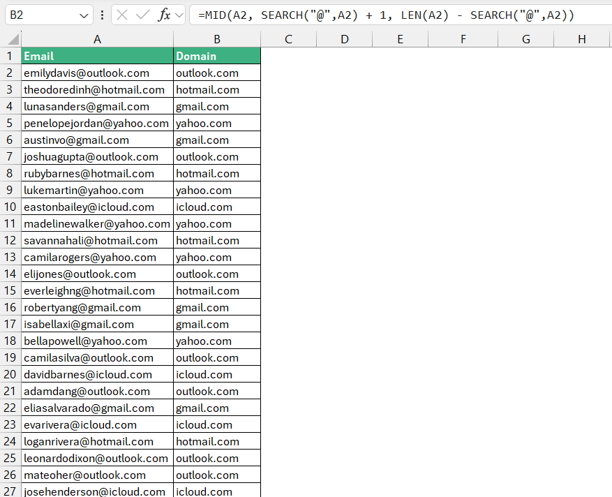
For domain names, if you wish to extract everything after the “@” symbol, the combination of MID and SEARCH functions become extremely useful:
=MID(email_cell, SEARCH("@", email_cell) + 1, LEN(email_cell) - SEARCH("@", email_cell))
This formula pinpoints the “@” position and pulls the remainder of the string, giving you the domain.
In essence, while domain names might appear as simple text entries, they’re actually structured information that can be deconstructed and understood through the lens of Excel’s string-manipulation functions.
Tips for Efficiently Cleaning Up Data
Combining TRIM, CLEAN, and SUBSTITUTE for Precision
In the realm of data cleaning, Excel’s TRIM, CLEAN, and SUBSTITUTE functions are the fine brushes you use to detail your dataset to perfection. When wielded together, they turn messy text into a standardized format that lends itself easily to analysis and reporting.
First up is TRIM, which sweeps away extra spaces except for single spaces between words. Applying =TRIM(A1) will neaten up any text by eliminating redundant spaces, ensuring consistency across your data.
Then there’s CLEAN, which delves deeper, removing non-printable characters that sometimes tag along when you import data from other sources. Cast =CLEAN(A1) to banish these invisible gremlins from your text.
SUBSTITUTE is the precision tool used to replace specific characters or text with alternatives or nothing at all. With =SUBSTITUTE(A1, "old_text", "new_text"), you update text strings with complete control, whether for updating URLs, correcting product codes, or standardizing terminology.
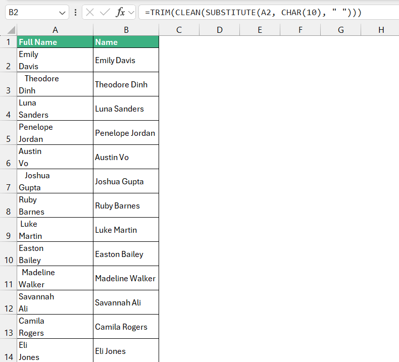
Imagine a scenario where you’ve imported a list peppered with irregular spacing and line breaks. By combining these functions:
=TRIM(CLEAN(SUBSTITUTE(A1, CHAR(10), " ")))
You first swap out line breaks with spaces using SUBSTITUTE and CHAR(10), then CLEAN steps in, and TRIM finishes the job, providing you with pristine text ready for use.
Mastering this trio will elevate the quality of your data, ensuring that when you move to analyze or report it, you do so with the highest level of clarity and precision.
One can’t understate the impact of starting your analytical process with spotless data—it not only saves time but also aligns with the adage: “garbage in, garbage out.”
Avoiding Common Pitfalls: Error Checking with IFERROR
When you’re knee-deep in Excel functions, there’s an ever-present risk of encountering error values that can derail your analysis. That’s where the IFERROR function becomes your safety net, allowing you to manage errors gracefully and keep your datasets clean.
IFERROR comes in handy when you anticipate potential errors in your formulas and wish to handle them proactively. Rather than display the standard error codes like #N/A, #VALUE!, or #REF!, you can decide what should appear in the cells when things go awry.
By wrapping your formula in IFERROR, you can specify a default value or text to be shown instead, like so:
=IFERROR(your_formula, "Error")
As well as maintaining aesthetics, IFERROR simplifies your troubleshooting process. Instead of weeding through numerous error values, you have a clear indication of where things aren’t going as planned.
Frequently Asked Questions (FAQs)
Q1: What is the easiest way to extract a specific word from a cell?
The simplest way is to use the left function such as =Left(A1, n) where A1 is the cell reference containing the text and n is the position of the word you want to extract. If you need any custom function, you’d typically employ a combination of Excel’s LEFT, RIGHT, MID, SEARCH, and TRIM functions.
Q2: How can I pull text that lies between two characters in Excel?
To extract text between two specific characters in Excel, use the MID and SEARCH functions together. For example, “=MID(A1, SEARCH(“first_char”, A1) + 1, SEARCH(“second_char”, A1) – SEARCH(“first_char”, A1) – 1)” where “A1” is the text source. Adjust “first_char” and “second_char” to match your case.
Q3: Is it possible to extract data based on variable positions within cells?
Yes, it’s possible to extract data based on variable positions within cells by using Excel’s SEARCH or FIND functions to locate the position of a specific character or substring, then applying MID, LEFT, or RIGHT functions to extract the data relative to that position.
Q4: Can I use substring functions to manipulate data outside of Excel?
Yes, while Excel substring functions are specific to Excel, the logic can be applied in other spreadsheet applications and programming languages that contain similar functions or string manipulation methods. However, the syntax may differ.
Q5: What is a substring?
A substring is a contiguous sequence of characters within a larger text string. In Excel, it’s part of a cell’s content that you can extract using various text functions, like LEFT, MID, or RIGHT.
John Michaloudis is a former accountant and finance analyst at General Electric, a Microsoft MVP since 2020, an Amazon #1 bestselling author of 4 Microsoft Excel books and teacher of Microsoft Excel & Office over at his flagship Academy Online Course.
