Field Name Formatting in Excel Pivot Tables

I will show you how to set up field name formatting in Excel Pivot Tables!

Exercise Workbook:

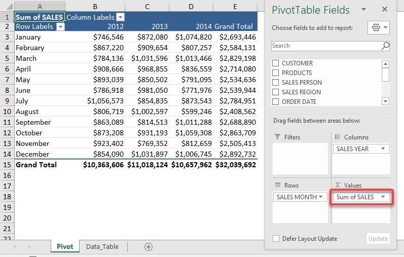
Here is our Pivot Table. We want to change the Sum of SALES to Total Sales for better readability.

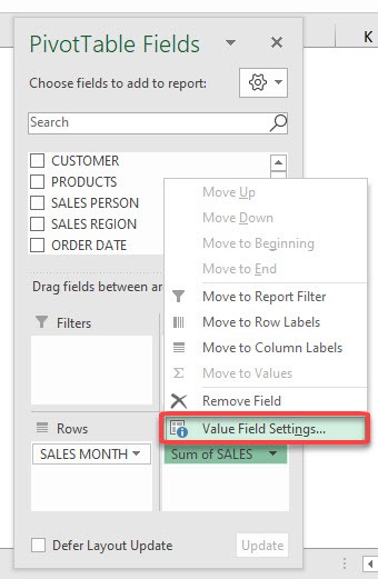
STEP 1: Click on the arrow beside Sum of SALES and select Value Field Settings

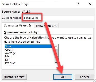
STEP 2: Type Total Sales for the Custom Name and click OK

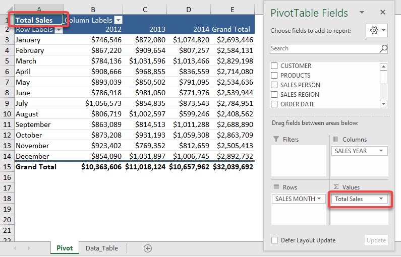
Now you have Total Sales as your Field Name!

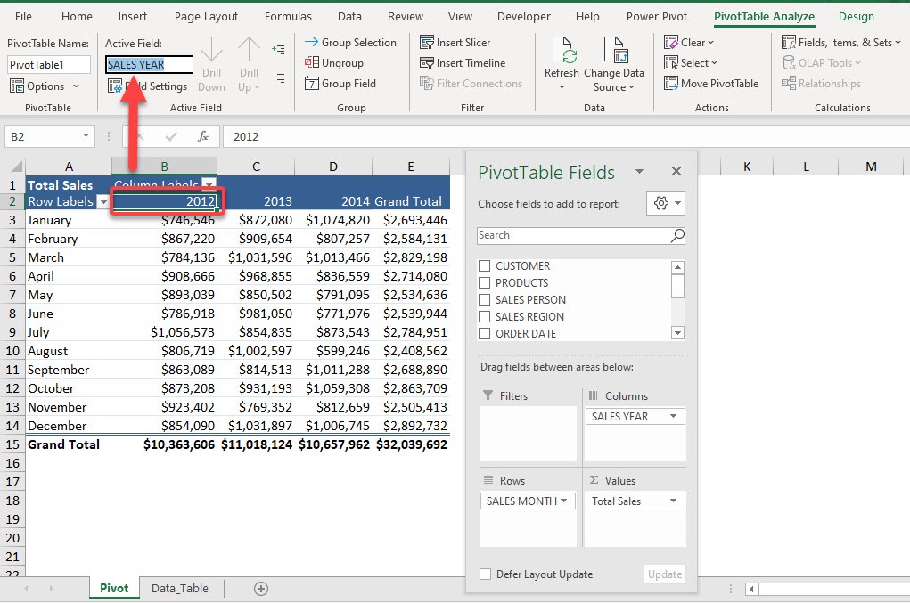
STEP 3: There is another way to do this. Now we want to change SALES YEAR to Financial Year

Select any SALES YEAR label in your Pivot Table. Go to PivotTable Analyze > Active Field > Active Field

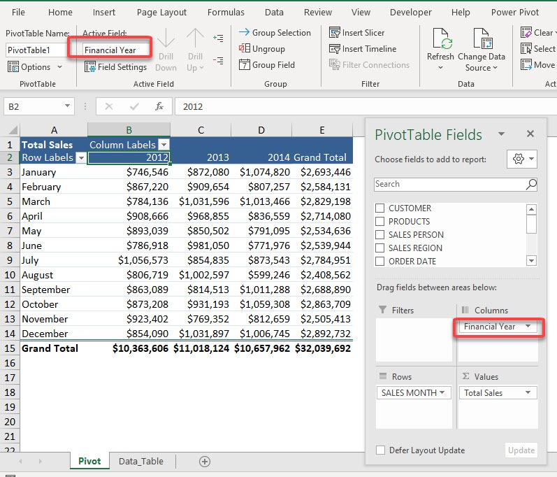
Type in Financial Year as the new name:

And you can see your new field name take effect!

Make sure to download our FREE PDF on the 333 Excel keyboard Shortcuts here:

Bryan

Bryan is a best-selling book author of the 101 Excel Series paperback books.